Section 9 7 Infinite Series Maclaurin and Taylor

Section 9. 7 Infinite Series: “Maclaurin and Taylor Polynomials”

All graphics are attributed to: Calculus, 10/E by Howard Anton, Irl Bivens, and Stephen Davis Copyright © 2009 by John Wiley & Sons, Inc. All rights reserved. ”

Introduction In a local linear approximation, the tangent line to the graph of a function is used to obtain a linear approximation of the function near the point of tangency. In this section, we will consider how one might improve on the accuracy of local linear approximations by using higher-order polynomials as approximating functions. We will also investigate the error associated with such approximations.

Local Linear Approximations

Local Quadratic Approximations

Substitution for Local Quadratic Approximation

Example

Maclaurin Polynomials Since the quadratic approximation was better than the local linear approximation, might a cubic or quartic (degree 4) approximation be better yet? To find out, we must extend our work on quadratics to a more general idea for higher degree polynomial approximations. See substitution work similar to that we did for quadratics on page 650 for higher degree polynomials.

Colin Maclaurin (1698 -1746)

Example

Analysis of Example Results

Example Find the nth Maclaurin polynomials for sin x. Solution: Start by finding several derivatives of sin x. f(x) = sin x f(0) = sin 0 = 0 f’(x) = cos x f’(0) = cos 0 = 1 f”(x) = -sin x f”(0) = -sin 0 = 0 f’’’(x) = -cos x f’’’(0) = -cos 0 = -1 f””(x) = sin x f””(0) = sin 0 = 0 and the pattern (0, 1, 0, -1) continues to repeat for further derivatives at 0.

Example continued

Graph of Example Results If you are interested, see the nth Maclaurin polynomials for cos x on page 652.

Taylor Polynomials

Brook Taylor (1685 -1731) Taylor polynomials are named after the English mathematician Brook Taylor who claims to have worked/conversed with Isaac Newton on planetary motion and Halley’s comet regarding roots of polynomials. Supposedly, his writing style was hard to understand did not receive credit for many of his innovations on a wide range of subjects – magnetism, capillary action, thermometers, perspective, and calculus. See more information on page 653. Remember, Maclaurin series came later and they are a more specific case of Taylor series.

Example

Example continued

Sigma Notation for Taylor and Maclaurin Polynomials

Example

Sigma Notation for a Taylor Polynomial The computations and substitutions are similar to those in the previous example except you use the more general form. See example 6 on page 655

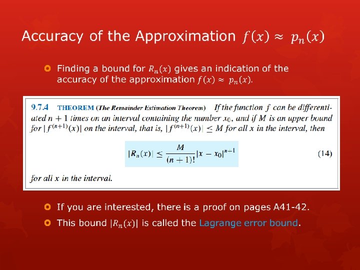
The n. TH Remainder

Example given accuracy

Example continued

Another Accuracy Example

Example continued

Getting Ready to Race