Search Heuristic Optimal Artificial Intelligence CMSC 25000 January

Search: Heuristic &Optimal Artificial Intelligence CMSC 25000 January 16, 2003

Agenda • Heuristic Search – Local: Hill-climbing, Beam Search • Limitations of local heuristics – Global: Best first • Optimal Search – A* search • Admissible, consistent heuristics • Dynamic programming • Problem representation

Searches • Blind search: Find ANY path to goal – Know something about search space: • Most paths reach goal or terminate quickly: DFS • Low branching factor, possible long paths: BFS • Always ready to act: ID-DFS

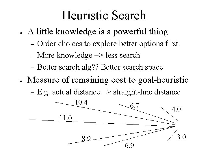
Heuristic Search ● A little knowledge is a powerful thing – – – ● Order choices to explore better options first More knowledge => less search Better search alg? ? Better search space Measure of remaining cost to goal-heuristic – E. g. actual distance => straight-line distance 10. 4 6. 7 4. 0 11. 0 8. 9 3. 0 6. 9

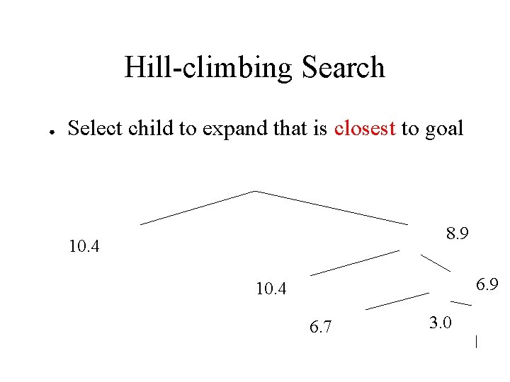
Hill-climbing Search ● Select child to expand that is closest to goal 8. 9 10. 4 6. 7 3. 0

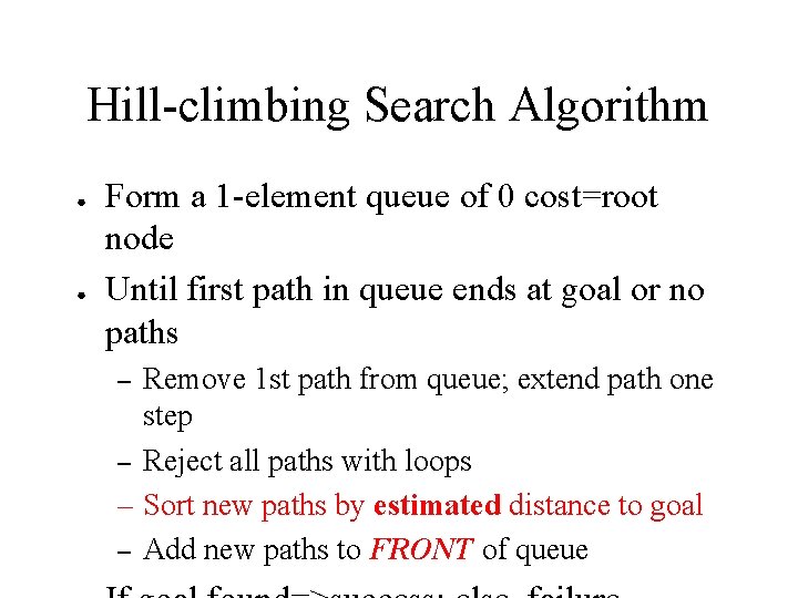
Hill-climbing Search Algorithm ● ● Form a 1 -element queue of 0 cost=root node Until first path in queue ends at goal or no paths Remove 1 st path from queue; extend path one step – Reject all paths with loops – Sort new paths by estimated distance to goal – Add new paths to FRONT of queue –

Beam Search ● Breadth-first search of fixed width - top w – Guarantees limited branching factor, E. g. w=2

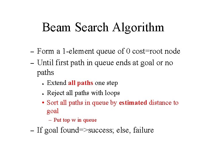
Beam Search Algorithm – – Form a 1 -element queue of 0 cost=root node Until first path in queue ends at goal or no paths Extend all paths one step ● Reject all paths with loops • Sort all paths in queue by estimated distance to goal ● – Put top w in queue – If goal found=>success; else, failure

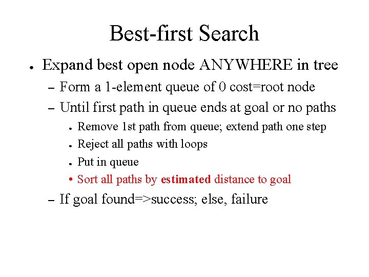
Best-first Search ● Expand best open node ANYWHERE in tree – – Form a 1 -element queue of 0 cost=root node Until first path in queue ends at goal or no paths Remove 1 st path from queue; extend path one step ● Reject all paths with loops ● Put in queue • Sort all paths by estimated distance to goal ● – If goal found=>success; else, failure

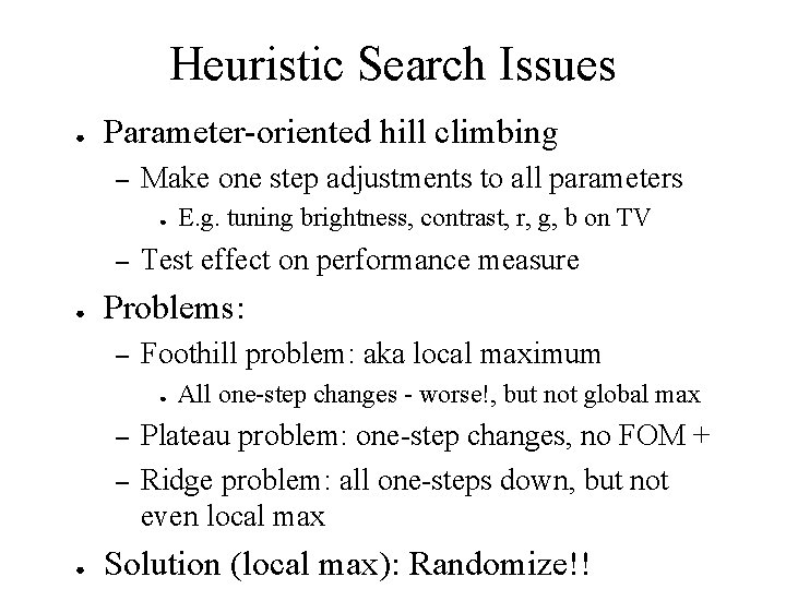
Heuristic Search Issues ● Parameter-oriented hill climbing – Make one step adjustments to all parameters ● – ● Test effect on performance measure Problems: – Foothill problem: aka local maximum ● – – ● E. g. tuning brightness, contrast, r, g, b on TV All one-step changes - worse!, but not global max Plateau problem: one-step changes, no FOM + Ridge problem: all one-steps down, but not even local max Solution (local max): Randomize!!

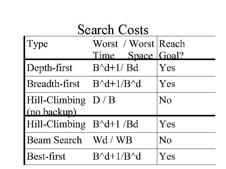
Search Costs

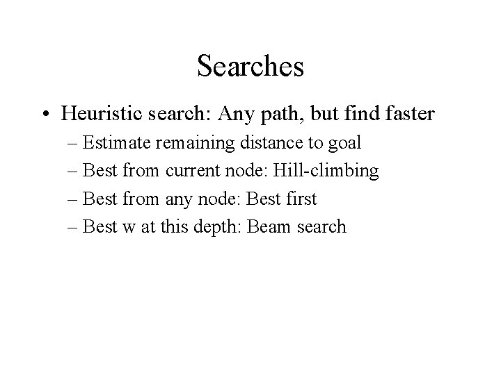
Searches • Heuristic search: Any path, but find faster – Estimate remaining distance to goal – Best from current node: Hill-climbing – Best from any node: Best first – Best w at this depth: Beam search

Optimal Search • Find BEST path to goal – Find best path EFFICIENTLY • Exhaustive search: – Try all paths: return best • Optimal paths with less work: – Expand shortest paths – Expanded shortest expected paths – Eliminate repeated work - dynamic programming

Efficient Optimal Search • Find best path without exploring all paths – Use knowledge about path lengths • Maintain path & path length – Expand shortest paths first – Halt if partial path length > complete path length

Underestimates • Improve estimate of complete path length – Add (under)estimate of remaining distance – u(total path dist) = d(partial path)+u(remaining) – Underestimates must ultimately yield shortest – Stop if all u(total path dist) > d(complete path) • Straight-line distance => underestimate • Better estimate => Better search • No missteps

Search with Dynamic Programming • Avoid duplicating work – Dynamic Programming principle: • Shortest path from S to G through I is shortest path from S to I plus shortest path from I to G • No need to consider other routes to or from I

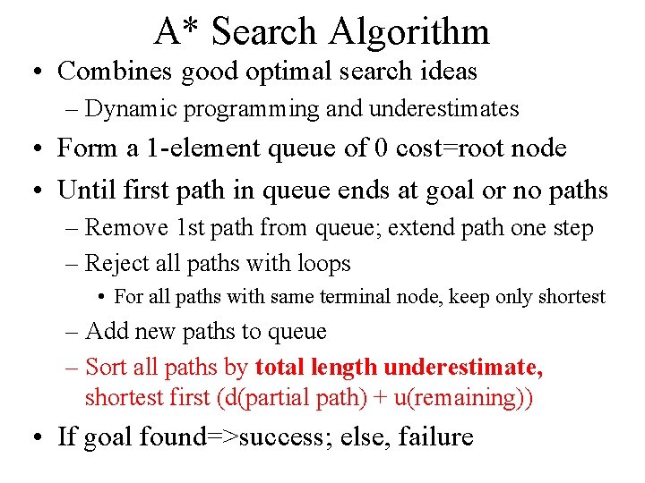
A* Search Algorithm • Combines good optimal search ideas – Dynamic programming and underestimates • Form a 1 -element queue of 0 cost=root node • Until first path in queue ends at goal or no paths – Remove 1 st path from queue; extend path one step – Reject all paths with loops • For all paths with same terminal node, keep only shortest – Add new paths to queue – Sort all paths by total length underestimate, shortest first (d(partial path) + u(remaining)) • If goal found=>success; else, failure

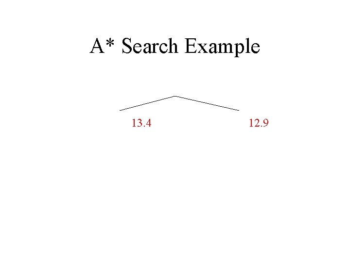
A* Search Example 13. 4 12. 9

Heuristics • A* search: only as good as the heuristic • Heuristic requirements: – Admissible: • UNDERESTIMATE true remaining cost to goal – Consistent: • h(n) <= c(n, a, n') + h(n') • Some heuristics better than others – 0?

Constructing Heuristics • Relaxation: – State problem – Remove one or more constraints • What is the cost then? • Example: – 8 -square: Move A to B if • 1) A &B horizontally or vertically adjacent, and • 2) B is empty – Ignore 1) -> Manhattan distance

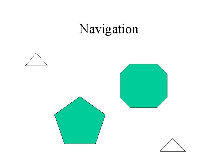
Navigation

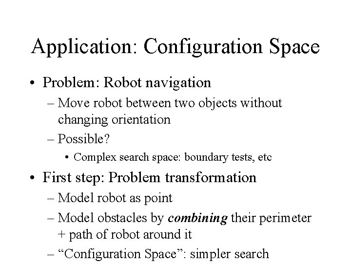
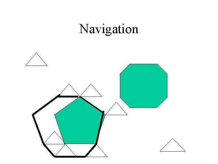
Application: Configuration Space • Problem: Robot navigation – Move robot between two objects without changing orientation – Possible? • Complex search space: boundary tests, etc • First step: Problem transformation – Model robot as point – Model obstacles by combining their perimeter + path of robot around it – “Configuration Space”: simpler search

Navigation

Navigation

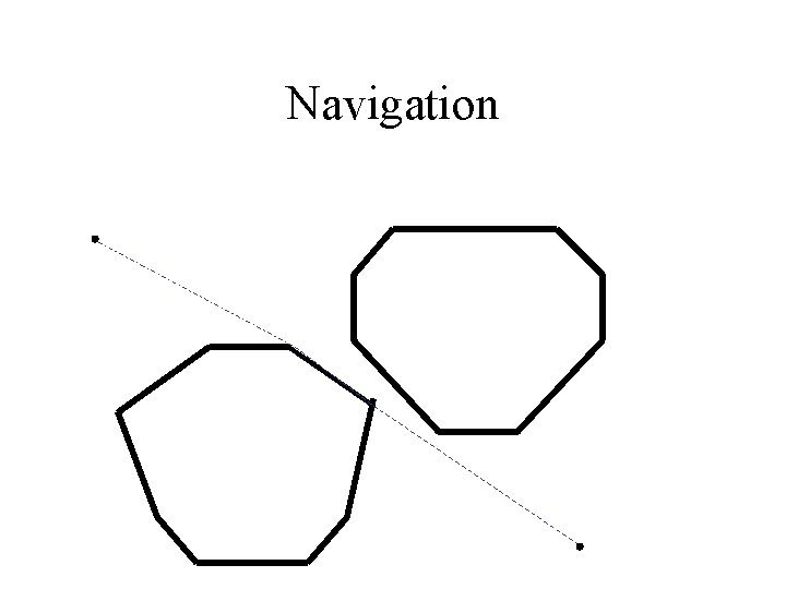
Navigation as Simple Search • Replace funny robot shape in field of funny shaped obstacles with – Point robot in field of configuration shapes • All movement is: – Start to vertex, vertex to vertex, or vertex to goal • Search: Start, vertices, goal, & connections • A* search yields efficient least cost path

Online Search • Offline search: – Think a lot, then act once • Online search: – Think a little, act, look, think, . . – Necessary for exploration, (semi)dynamic env – Components: Actions, step-cost, goal test – Compare cost to optimal if env known • Competitive ratio (possibly infinite)

Online Search Agents • Exploration: – Perform action in state -> record result – Search locally • Why? DFS? BFS? • Backtracking requires reversibility – Strategy: Hill-climb • Use memory: if stuck, try apparent best neighbor • Unexplored state: assume closest – Encourages exploration

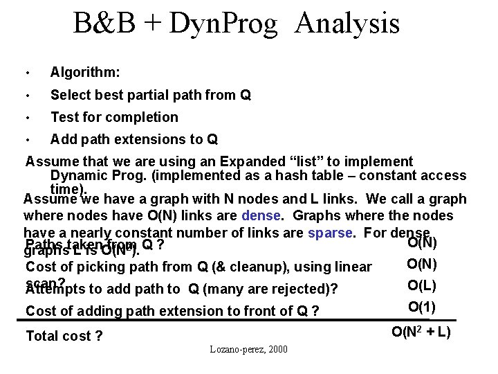
B&B + Dyn. Prog Analysis • Algorithm: • Select best partial path from Q • Test for completion • Add path extensions to Q Assume that we are using an Expanded “list” to implement Dynamic Prog. (implemented as a hash table – constant access time). Assume we have a graph with N nodes and L links. We call a graph where nodes have O(N) links are dense. Graphs where the nodes have a nearly constant number of links are sparse. For dense O(N) Paths taken from 2). Q ? graphs L is O(N) Cost of picking path from Q (& cleanup), using linear scan? O(L) Attempts to add path to Q (many are rejected)? Cost of adding path extension to front of Q ? O(1) O(N 2 + L) Total cost ? Lozano-perez, 2000

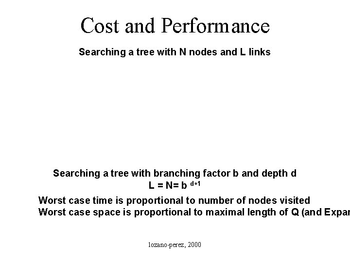
Cost and Performance Searching a tree with N nodes and L links Searching a tree with branching factor b and depth d L = N= b d+1 Worst case time is proportional to number of nodes visited Worst case space is proportional to maximal length of Q (and Expan lozano-perez, 2000