Uncertain Reasoning over Time Artificial Intelligence CMSC 25000

Uncertain Reasoning over Time Artificial Intelligence CMSC 25000 February 22, 2007

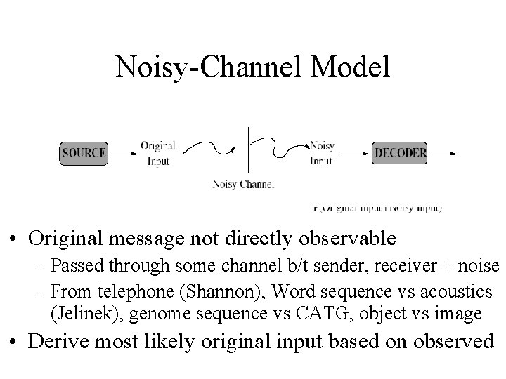
Noisy-Channel Model • Original message not directly observable – Passed through some channel b/t sender, receiver + noise – From telephone (Shannon), Word sequence vs acoustics (Jelinek), genome sequence vs CATG, object vs image • Derive most likely original input based on observed

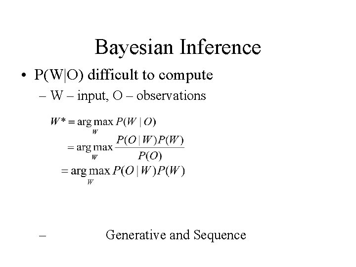
Bayesian Inference • P(W|O) difficult to compute – W – input, O – observations – Generative and Sequence

Applications • AI: Speech recognition!, POS tagging, sense tagging, dialogue, image understanding, information retrieval • Non-AI: – Bioinformatics: gene sequencing – Security: intrusion detection – Cryptography

Hidden Markov Models: Probabilistic Reasoning Over Time Natural Language Processing CMSC 25000 February 22, 2007

Agenda • Hidden Markov Models – Uncertain observation – Temporal Context – Recognition: Viterbi – Training the model: Baum-Welch • Speech Recognition – Framing the problem: Sounds to Sense – Speech Recognition as Modern AI

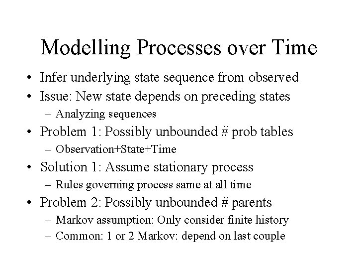
Modelling Processes over Time • Infer underlying state sequence from observed • Issue: New state depends on preceding states – Analyzing sequences • Problem 1: Possibly unbounded # prob tables – Observation+State+Time • Solution 1: Assume stationary process – Rules governing process same at all time • Problem 2: Possibly unbounded # parents – Markov assumption: Only consider finite history – Common: 1 or 2 Markov: depend on last couple

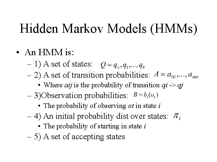
Hidden Markov Models (HMMs) • An HMM is: – 1) A set of states: – 2) A set of transition probabilities: • Where aij is the probability of transition qi -> qj – 3)Observation probabilities: • The probability of observing ot in state i – 4) An initial probability dist over states: • The probability of starting in state i – 5) A set of accepting states

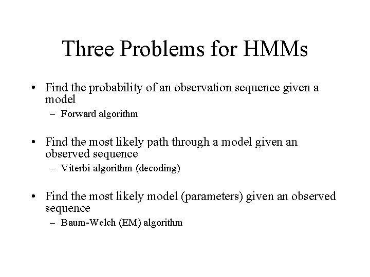
Three Problems for HMMs • Find the probability of an observation sequence given a model – Forward algorithm • Find the most likely path through a model given an observed sequence – Viterbi algorithm (decoding) • Find the most likely model (parameters) given an observed sequence – Baum-Welch (EM) algorithm

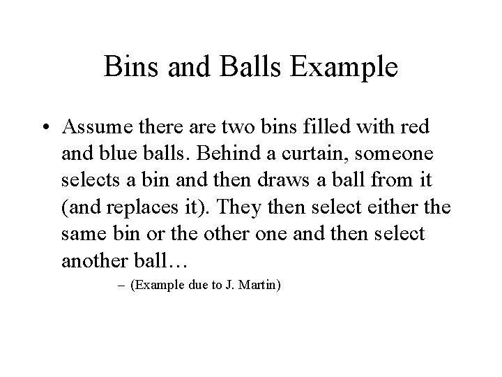
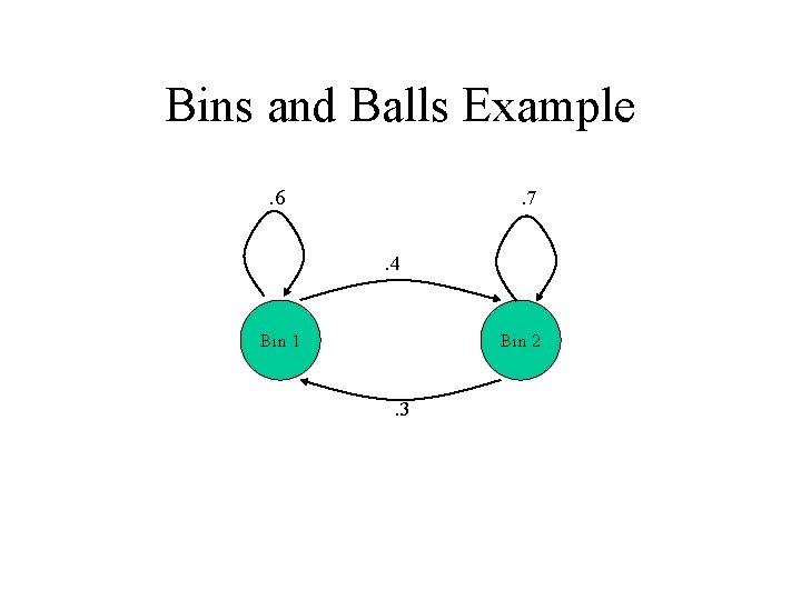
Bins and Balls Example • Assume there are two bins filled with red and blue balls. Behind a curtain, someone selects a bin and then draws a ball from it (and replaces it). They then select either the same bin or the other one and then select another ball… – (Example due to J. Martin)

Bins and Balls Example. 6 . 7. 4 Bin 1 Bin 2 . 3

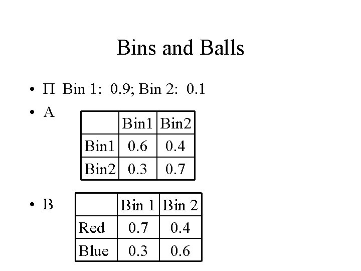
Bins and Balls • Π Bin 1: 0. 9; Bin 2: 0. 1 • A Bin 1 Bin 2 Bin 1 0. 6 0. 4 Bin 2 0. 3 0. 7 • B Bin 1 Bin 2 Red 0. 7 0. 4 Blue 0. 3 0. 6

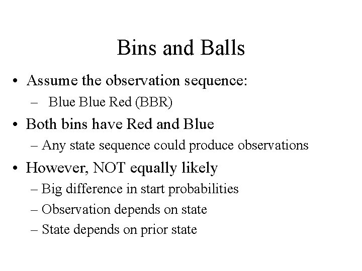
Bins and Balls • Assume the observation sequence: – Blue Red (BBR) • Both bins have Red and Blue – Any state sequence could produce observations • However, NOT equally likely – Big difference in start probabilities – Observation depends on state – State depends on prior state

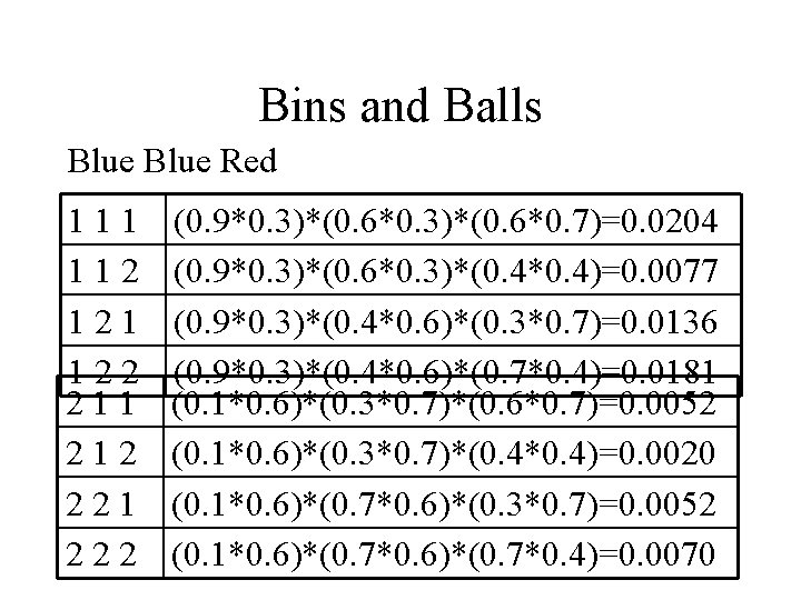
Bins and Balls Blue Red 111 112 121 122 211 212 221 222 (0. 9*0. 3)*(0. 6*0. 7)=0. 0204 (0. 9*0. 3)*(0. 6*0. 3)*(0. 4*0. 4)=0. 0077 (0. 9*0. 3)*(0. 4*0. 6)*(0. 3*0. 7)=0. 0136 (0. 9*0. 3)*(0. 4*0. 6)*(0. 7*0. 4)=0. 0181 (0. 1*0. 6)*(0. 3*0. 7)*(0. 6*0. 7)=0. 0052 (0. 1*0. 6)*(0. 3*0. 7)*(0. 4*0. 4)=0. 0020 (0. 1*0. 6)*(0. 7*0. 6)*(0. 3*0. 7)=0. 0052 (0. 1*0. 6)*(0. 7*0. 4)=0. 0070

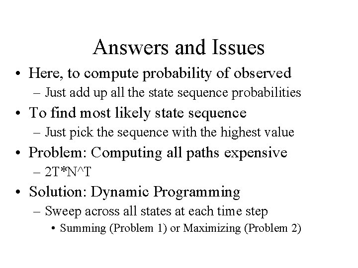
Answers and Issues • Here, to compute probability of observed – Just add up all the state sequence probabilities • To find most likely state sequence – Just pick the sequence with the highest value • Problem: Computing all paths expensive – 2 T*N^T • Solution: Dynamic Programming – Sweep across all states at each time step • Summing (Problem 1) or Maximizing (Problem 2)

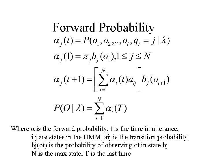
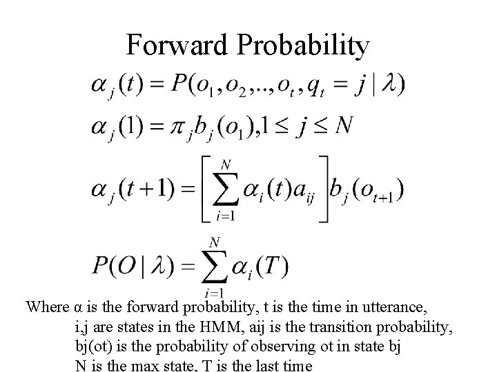
Forward Probability Where α is the forward probability, t is the time in utterance, i, j are states in the HMM, aij is the transition probability, bj(ot) is the probability of observing ot in state bj N is the max state, T is the last time

Forward Algorithm • Idea: matrix where each cell forward[t, j] represents probability of being in state j after seeing first t observations. • Each cell expresses the probability: forward[t, j] = P(o 1, o 2, . . . , ot, qt=j|w) • qt = j means "the probability that the tth state in the sequence of states is state j. • Compute probability by summing over extensions of all paths leading to current cell. • An extension of a path from a state i at time t-1 to state j at t is computed by multiplying together: i. previous path probability from the previous cell forward[t 1, i], ii. transition probability aij from previous state i to current state j iii. observation likelihood bjt that current state j matches observation symbol t.

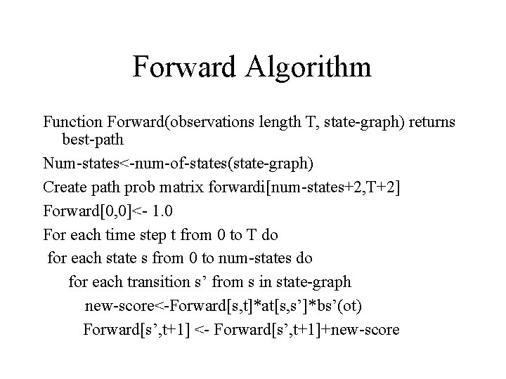
Forward Algorithm Function Forward(observations length T, state-graph) returns best-path Num-states<-num-of-states(state-graph) Create path prob matrix forwardi[num-states+2, T+2] Forward[0, 0]<- 1. 0 For each time step t from 0 to T do for each state s from 0 to num-states do for each transition s’ from s in state-graph new-score<-Forward[s, t]*at[s, s’]*bs’(ot) Forward[s’, t+1] <- Forward[s’, t+1]+new-score

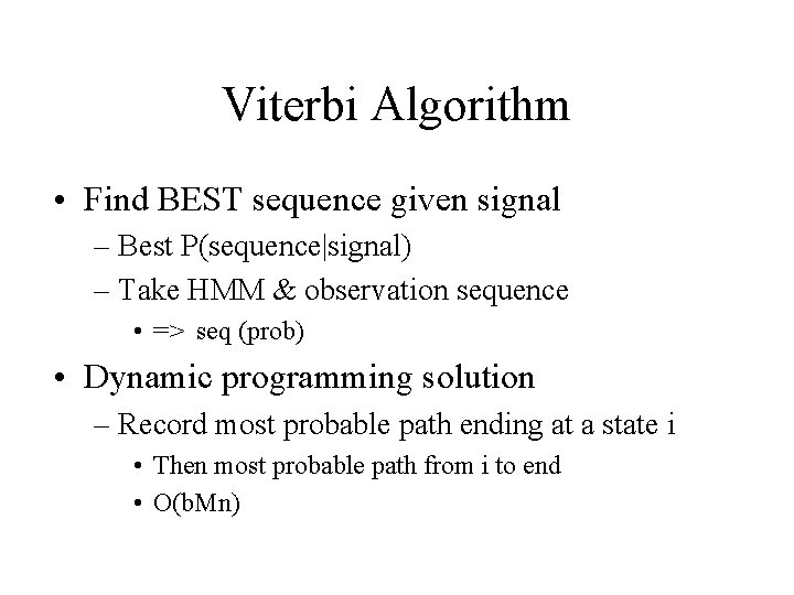
Viterbi Algorithm • Find BEST sequence given signal – Best P(sequence|signal) – Take HMM & observation sequence • => seq (prob) • Dynamic programming solution – Record most probable path ending at a state i • Then most probable path from i to end • O(b. Mn)

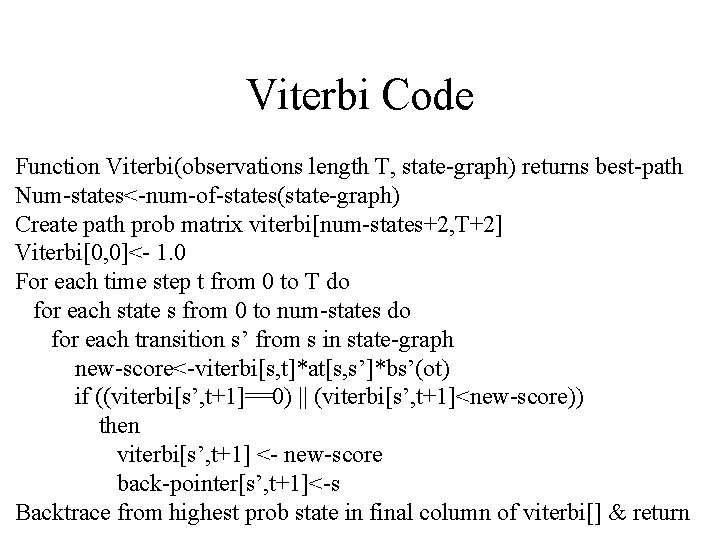
Viterbi Code Function Viterbi(observations length T, state-graph) returns best-path Num-states<-num-of-states(state-graph) Create path prob matrix viterbi[num-states+2, T+2] Viterbi[0, 0]<- 1. 0 For each time step t from 0 to T do for each state s from 0 to num-states do for each transition s’ from s in state-graph new-score<-viterbi[s, t]*at[s, s’]*bs’(ot) if ((viterbi[s’, t+1]==0) || (viterbi[s’, t+1]<new-score)) then viterbi[s’, t+1] <- new-score back-pointer[s’, t+1]<-s Backtrace from highest prob state in final column of viterbi[] & return

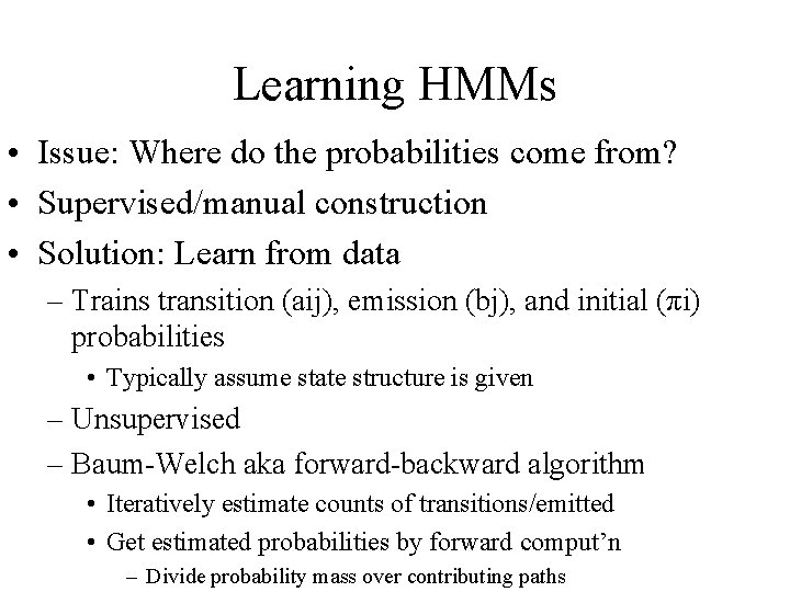
Learning HMMs • Issue: Where do the probabilities come from? • Supervised/manual construction • Solution: Learn from data – Trains transition (aij), emission (bj), and initial (πi) probabilities • Typically assume state structure is given – Unsupervised – Baum-Welch aka forward-backward algorithm • Iteratively estimate counts of transitions/emitted • Get estimated probabilities by forward comput’n – Divide probability mass over contributing paths

Manual Construction • Manually labeled data – Observation sequences, aligned to – Ground truth state sequences • • • Compute (relative) frequencies of state transitions Compute frequencies of observations/state Compute frequencies of initial states Bootstrapping: iterate tag, correct, reestimate, tag. Problem: – Labeled data is expensive, hard/impossible to obtain, may be inadequate to fully estimate • Sparseness problems

Unsupervised Learning • Re-estimation from unlabeled data – Baum-Welch aka forward-backward algorithm – Assume “representative” collection of data • E. g. recorded speech, gene sequences, etc – Assign initial probabilities • Or estimate from very small labeled sample – Compute state sequences given the data • I. e. use forward algorithm – Update transition, emission, initial probabilities

Updating Probabilities • Intuition: – Observations identify state sequences – Adjust probability of transitions/emissions – Make closer to those consistent with observed – Increase P(Observations|Model) • Functionally – For each state i, what proportion of transitions from state i go to state j – For each state i, what proportion of observations match O? – How often is state i the initial state?

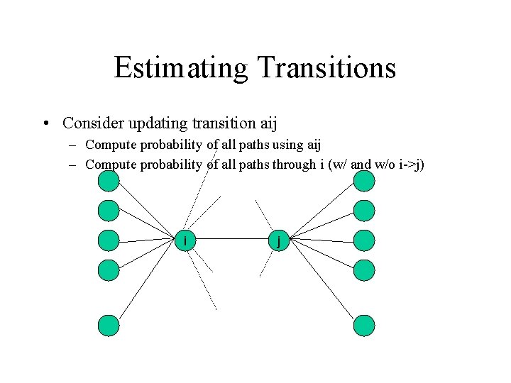
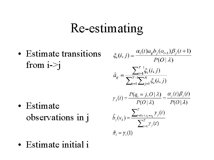
Estimating Transitions • Consider updating transition aij – Compute probability of all paths using aij – Compute probability of all paths through i (w/ and w/o i->j) i j

Forward Probability Where α is the forward probability, t is the time in utterance, i, j are states in the HMM, aij is the transition probability, bj(ot) is the probability of observing ot in state bj N is the max state, T is the last time

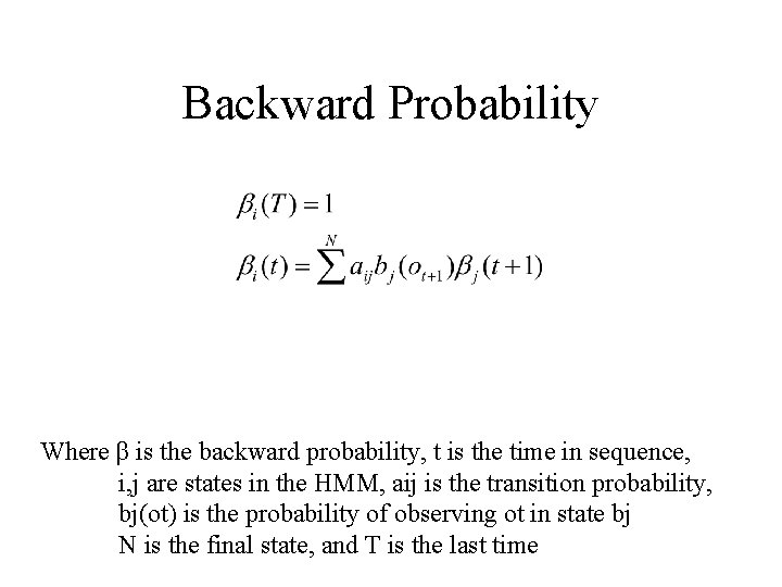
Backward Probability Where β is the backward probability, t is the time in sequence, i, j are states in the HMM, aij is the transition probability, bj(ot) is the probability of observing ot in state bj N is the final state, and T is the last time

Re-estimating • Estimate transitions from i->j • Estimate observations in j • Estimate initial i

Speech Recognition • Goal: – Given an acoustic signal, identify the sequence of words that produced it – Speech understanding goal: • Given an acoustic signal, identify the meaning intended by the speaker • Issues: – Ambiguity: many possible pronunciations, – Uncertainty: what signal, what word/sense produced this sound sequence

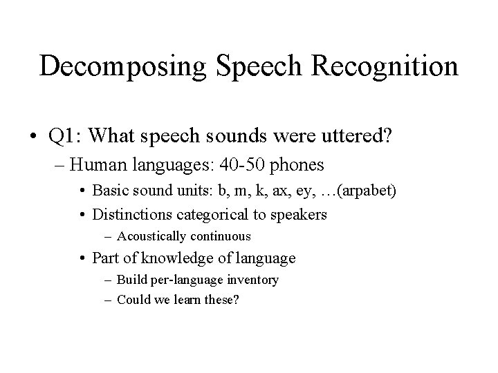
Decomposing Speech Recognition • Q 1: What speech sounds were uttered? – Human languages: 40 -50 phones • Basic sound units: b, m, k, ax, ey, …(arpabet) • Distinctions categorical to speakers – Acoustically continuous • Part of knowledge of language – Build per-language inventory – Could we learn these?

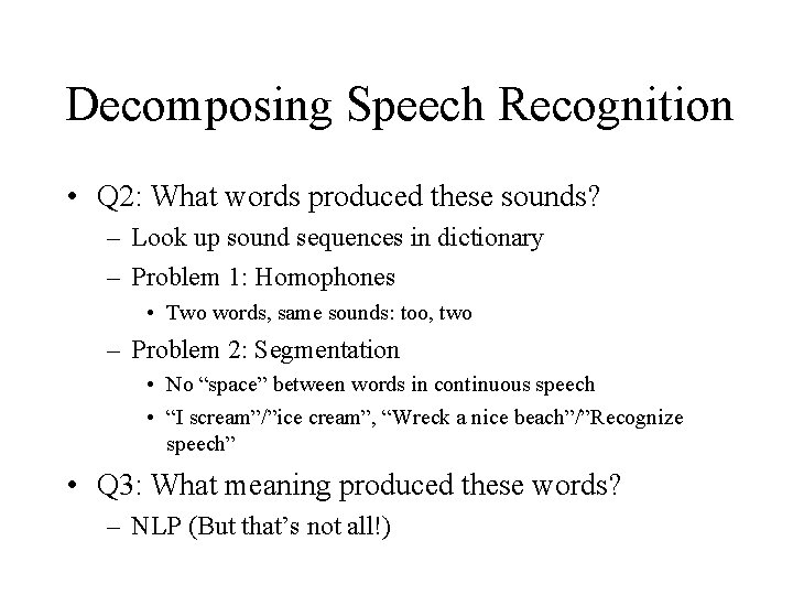
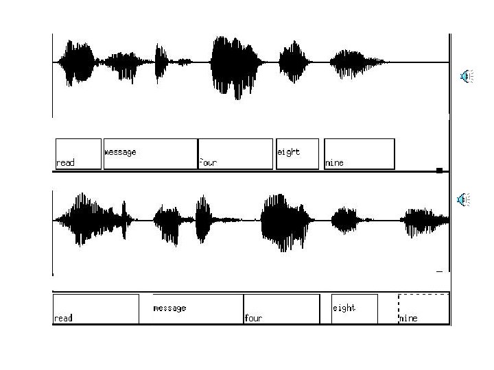
Decomposing Speech Recognition • Q 2: What words produced these sounds? – Look up sound sequences in dictionary – Problem 1: Homophones • Two words, same sounds: too, two – Problem 2: Segmentation • No “space” between words in continuous speech • “I scream”/”ice cream”, “Wreck a nice beach”/”Recognize speech” • Q 3: What meaning produced these words? – NLP (But that’s not all!)

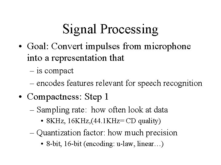
Signal Processing • Goal: Convert impulses from microphone into a representation that – is compact – encodes features relevant for speech recognition • Compactness: Step 1 – Sampling rate: how often look at data • 8 KHz, 16 KHz, (44. 1 KHz= CD quality) – Quantization factor: how much precision • 8 -bit, 16 -bit (encoding: u-law, linear…)

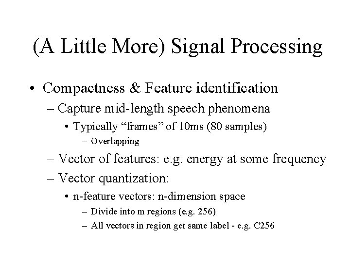
(A Little More) Signal Processing • Compactness & Feature identification – Capture mid-length speech phenomena • Typically “frames” of 10 ms (80 samples) – Overlapping – Vector of features: e. g. energy at some frequency – Vector quantization: • n-feature vectors: n-dimension space – Divide into m regions (e. g. 256) – All vectors in region get same label - e. g. C 256

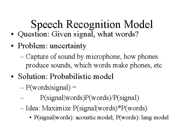
Speech Recognition Model • Question: Given signal, what words? • Problem: uncertainty – Capture of sound by microphone, how phones produce sounds, which words make phones, etc • Solution: Probabilistic model – P(words|signal) = – P(signal|words)P(words)/P(signal) – Idea: Maximize P(signal|words)*P(words) • P(signal|words): acoustic model; P(words): lang model

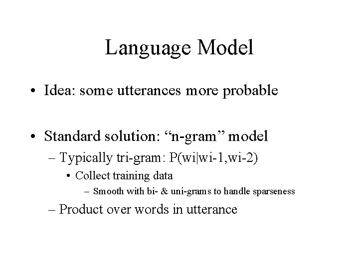
Language Model • Idea: some utterances more probable • Standard solution: “n-gram” model – Typically tri-gram: P(wi|wi-1, wi-2) • Collect training data – Smooth with bi- & uni-grams to handle sparseness – Product over words in utterance

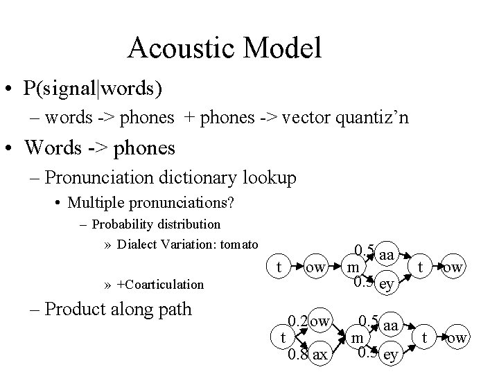
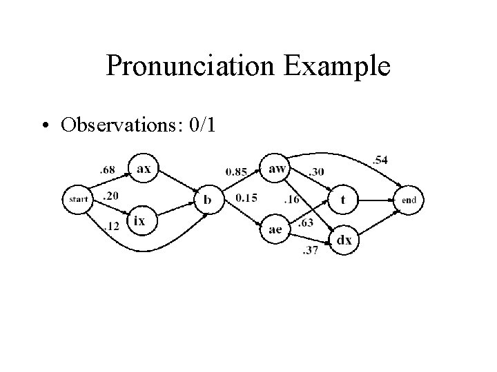
Acoustic Model • P(signal|words) – words -> phones + phones -> vector quantiz’n • Words -> phones – Pronunciation dictionary lookup • Multiple pronunciations? – Probability distribution » Dialect Variation: tomato t ow » +Coarticulation – Product along path t 0. 2 ow 0. 8 ax 0. 5 aa m 0. 5 ey t ow

Pronunciation Example • Observations: 0/1

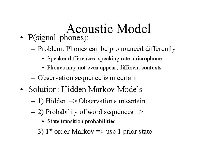
Acoustic Model • P(signal| phones): – Problem: Phones can be pronounced differently • Speaker differences, speaking rate, microphone • Phones may not even appear, different contexts – Observation sequence is uncertain • Solution: Hidden Markov Models – 1) Hidden => Observations uncertain – 2) Probability of word sequences => • State transition probabilities – 3) 1 st order Markov => use 1 prior state

Acoustic Model • 3 -state phone model for [m] – Use Hidden Markov Model (HMM) 0. 3 0. 9 0. 4 Transition probabilities Onset 0. 7 Mid 0. 1 End 0. 6 Final C 3: C 1: C 2: 0. 3 0. 5 0. 2 C 5: C 3: C 4: 0. 1 0. 2 0. 7 C 6: C 4: C 6: 0. 4 0. 1 0. 5 Observation probabilities – Probability of sequence: sum of prob of paths

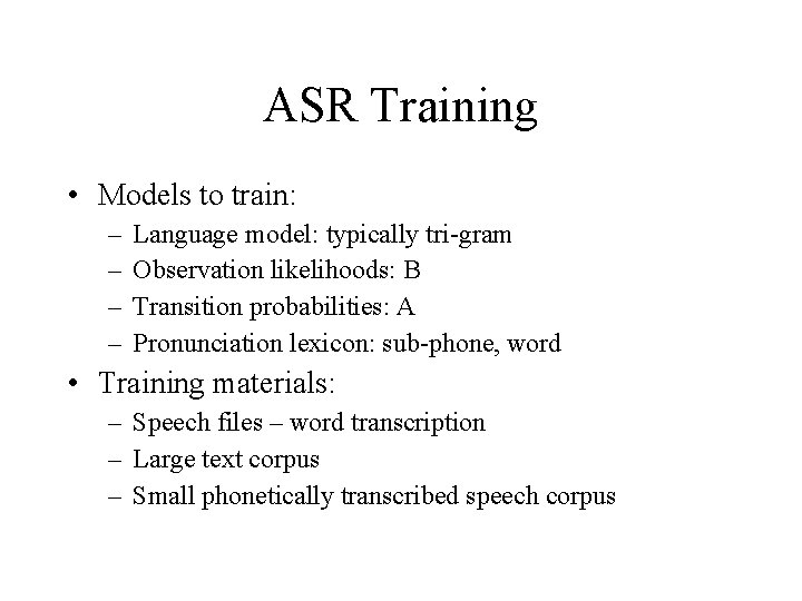
ASR Training • Models to train: – – Language model: typically tri-gram Observation likelihoods: B Transition probabilities: A Pronunciation lexicon: sub-phone, word • Training materials: – Speech files – word transcription – Large text corpus – Small phonetically transcribed speech corpus

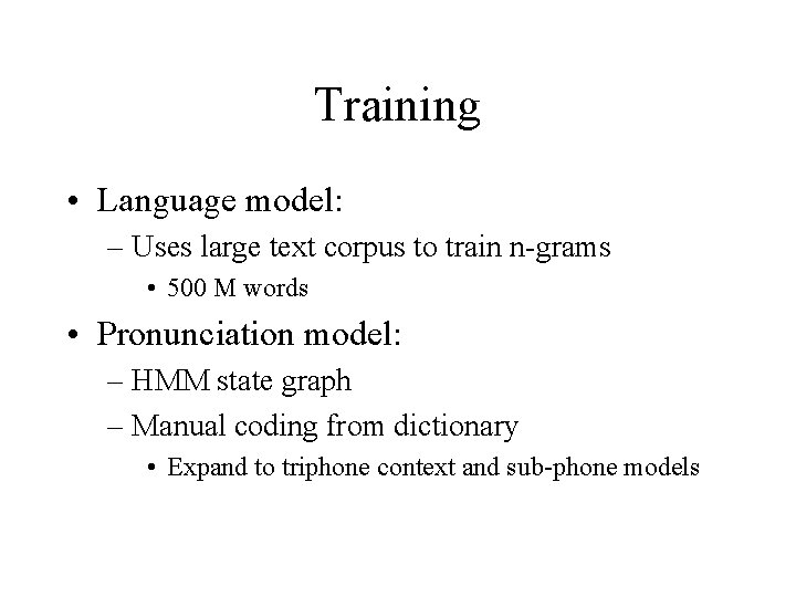
Training • Language model: – Uses large text corpus to train n-grams • 500 M words • Pronunciation model: – HMM state graph – Manual coding from dictionary • Expand to triphone context and sub-phone models

HMM Training • Training the observations: – E. g. Gaussian: set uniform initial mean/variance • Train based on contents of small (e. g. 4 hr) phonetically labeled speech set (e. g. Switchboard) • Training A&B: – Forward-Backward algorithm training

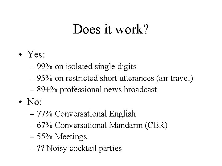
Does it work? • Yes: – 99% on isolated single digits – 95% on restricted short utterances (air travel) – 89+% professional news broadcast • No: – 77% Conversational English – 67% Conversational Mandarin (CER) – 55% Meetings – ? ? Noisy cocktail parties

N-grams • Perspective: – Some sequences (words/chars) are more likely than others – Given sequence, can guess most likely next • Used in – Speech recognition – Spelling correction, – Augmentative communication – Other NL applications

Probabilistic Language Generation • Coin-flipping models – A sentence is generated by a randomized algorithm • The generator can be in one of several “states” • Flip coins to choose the next state. • Flip other coins to decide which letter or word to output

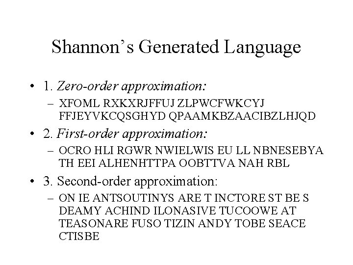
Shannon’s Generated Language • 1. Zero-order approximation: – XFOML RXKXRJFFUJ ZLPWCFWKCYJ FFJEYVKCQSGHYD QPAAMKBZAACIBZLHJQD • 2. First-order approximation: – OCRO HLI RGWR NWIELWIS EU LL NBNESEBYA TH EEI ALHENHTTPA OOBTTVA NAH RBL • 3. Second-order approximation: – ON IE ANTSOUTINYS ARE T INCTORE ST BE S DEAMY ACHIND ILONASIVE TUCOOWE AT TEASONARE FUSO TIZIN ANDY TOBE SEACE CTISBE

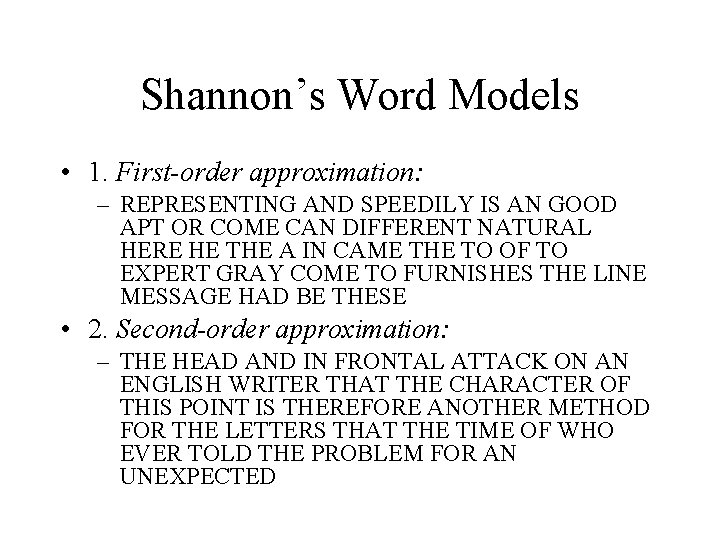
Shannon’s Word Models • 1. First-order approximation: – REPRESENTING AND SPEEDILY IS AN GOOD APT OR COME CAN DIFFERENT NATURAL HERE HE THE A IN CAME THE TO OF TO EXPERT GRAY COME TO FURNISHES THE LINE MESSAGE HAD BE THESE • 2. Second-order approximation: – THE HEAD AND IN FRONTAL ATTACK ON AN ENGLISH WRITER THAT THE CHARACTER OF THIS POINT IS THEREFORE ANOTHER METHOD FOR THE LETTERS THAT THE TIME OF WHO EVER TOLD THE PROBLEM FOR AN UNEXPECTED

Corpus Counts • Estimate probabilities by counts in large collections of text/speech • Issues: – Wordforms (surface) vs lemma (root) – Case? Punctuation? Disfluency? – Type (distinct words) vs Token (total)

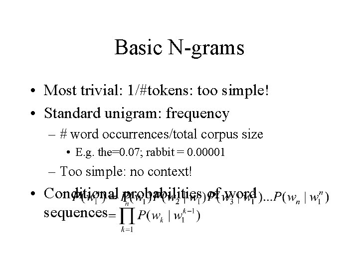
Basic N-grams • Most trivial: 1/#tokens: too simple! • Standard unigram: frequency – # word occurrences/total corpus size • E. g. the=0. 07; rabbit = 0. 00001 – Too simple: no context! • Conditional probabilities of word sequences

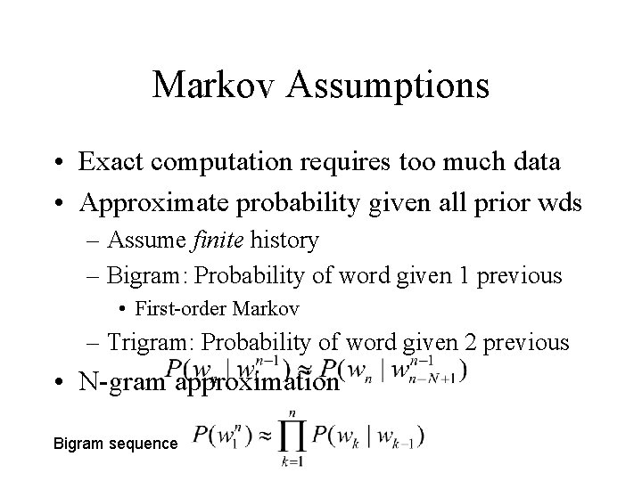
Markov Assumptions • Exact computation requires too much data • Approximate probability given all prior wds – Assume finite history – Bigram: Probability of word given 1 previous • First-order Markov – Trigram: Probability of word given 2 previous • N-gram approximation Bigram sequence

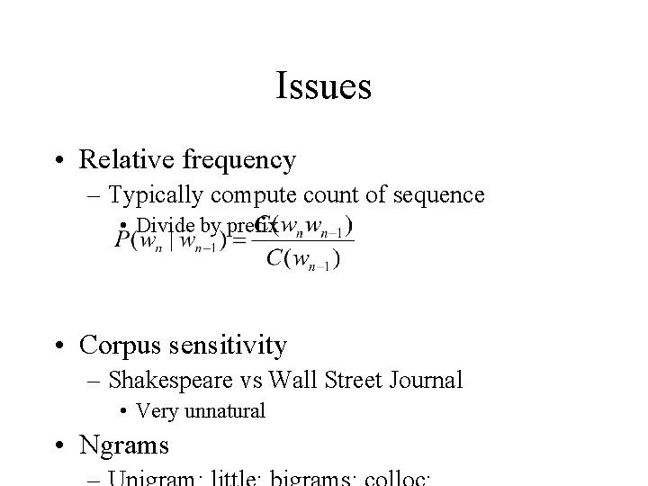
Issues • Relative frequency – Typically compute count of sequence • Divide by prefix • Corpus sensitivity – Shakespeare vs Wall Street Journal • Very unnatural • Ngrams

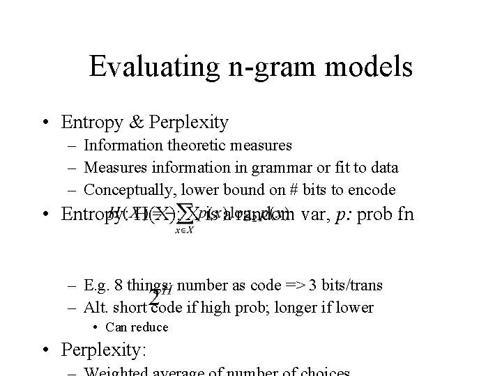
Evaluating n-gram models • Entropy & Perplexity – Information theoretic measures – Measures information in grammar or fit to data – Conceptually, lower bound on # bits to encode • Entropy: H(X): X is a random var, p: prob fn – E. g. 8 things: number as code => 3 bits/trans – Alt. short code if high prob; longer if lower • Can reduce • Perplexity:

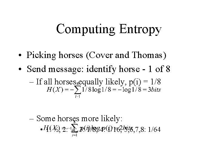
Computing Entropy • Picking horses (Cover and Thomas) • Send message: identify horse - 1 of 8 – If all horses equally likely, p(i) = 1/8 – Some horses more likely: • 1: ½; 2: ¼; 3: 1/8; 4: 1/16; 5, 6, 7, 8: 1/64

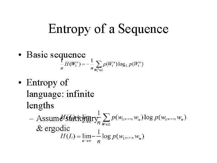
Entropy of a Sequence • Basic sequence • Entropy of language: infinite lengths – Assume stationary & ergodic

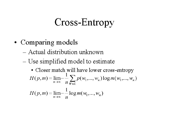
Cross-Entropy • Comparing models – Actual distribution unknown – Use simplified model to estimate • Closer match will have lower cross-entropy

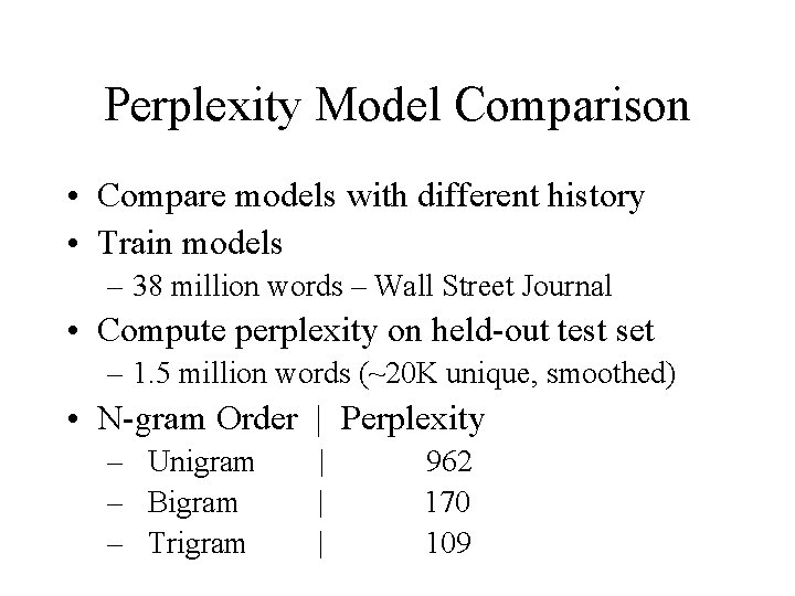
Perplexity Model Comparison • Compare models with different history • Train models – 38 million words – Wall Street Journal • Compute perplexity on held-out test set – 1. 5 million words (~20 K unique, smoothed) • N-gram Order | Perplexity – Unigram – Bigram – Trigram | | | 962 170 109

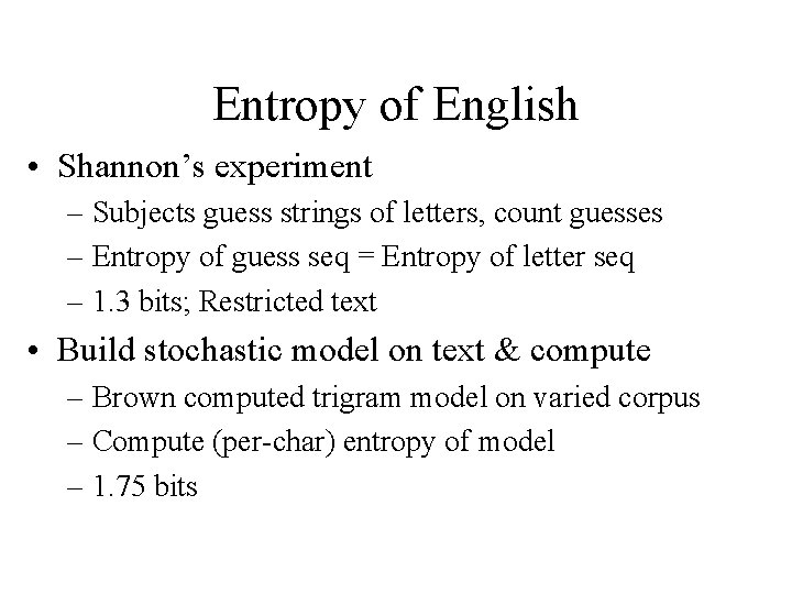
Entropy of English • Shannon’s experiment – Subjects guess strings of letters, count guesses – Entropy of guess seq = Entropy of letter seq – 1. 3 bits; Restricted text • Build stochastic model on text & compute – Brown computed trigram model on varied corpus – Compute (per-char) entropy of model – 1. 75 bits

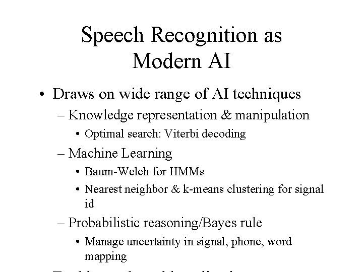
Speech Recognition as Modern AI • Draws on wide range of AI techniques – Knowledge representation & manipulation • Optimal search: Viterbi decoding – Machine Learning • Baum-Welch for HMMs • Nearest neighbor & k-means clustering for signal id – Probabilistic reasoning/Bayes rule • Manage uncertainty in signal, phone, word mapping