Search Optimal Artificial Intelligence CMSC 25000 January 2002

Search: Optimal Artificial Intelligence CMSC 25000 January, 2002

Agenda • Optimal vs Blind vs Heuristic Search • Optimal Search – All paths: British Museum procedure – Branch & Bound Search • Dynamic Programming • A* search • Problem representation – Configuration space

Searches • Blind search: Find ANY path to goal – Know nothing: Randomized seach – Know something about search space: • Most paths reach goal or terminate quickly: DFS • Low branching factor, possible long paths: BFS • Heuristic search: Any path, but find faster – Estimate remaining distance to goal – Best from current node: Hill-climbing – Best from any node: Best first – Best w at this depth: Beam search

Optimal Search • Find BEST path to goal – Find best path EFFICIENTLY • Exhaustive search: – Try all paths: return best • Optimal paths with less work: – Expand shortest paths – Expanded shortest expected paths – Eliminate repeated work - dynamic programming

British Museum Procedure • Explore all paths – Return the shortest – Perform DFS or BFS to traverse WHOLE tree • Expensive!!!! – Depth=d; Branching = b: b^d leaf nodes (paths) – Practical only for toy problems

Efficient Optimal Search • Find best path without exploring all paths – Use knowledge about path lengths • Maintain path & path length – Expand shortest paths first – Halt if partial path length > complete path length • Branch & Bound Search

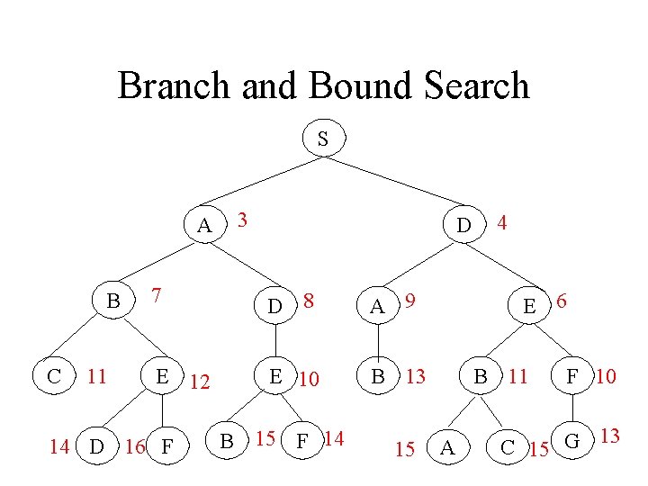
Branch and Bound Search S A B C 11 3 D 7 D 8 A 9 E 12 E 10 B 13 14 D 16 F B 15 F 14 15 4 E 6 B 11 A F 10 13 C 15 G

Branch & Bound Algorithm • Form a 1 -element queue of 0 cost=root node • Until first path in queue ends at goal or no paths – Remove 1 st path from queue; extend path one step – Reject all paths with loops – Add new paths to queue – Sort all paths by length, shortest first • If goal found=>success; else, failure

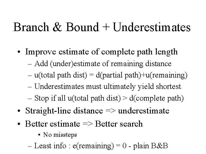
Branch & Bound + Underestimates • Improve estimate of complete path length – Add (under)estimate of remaining distance – u(total path dist) = d(partial path)+u(remaining) – Underestimates must ultimately yield shortest – Stop if all u(total path dist) > d(complete path) • Straight-line distance => underestimate • Better estimate => Better search • No missteps – Least info : e(remaining) = 0 - plain B&B

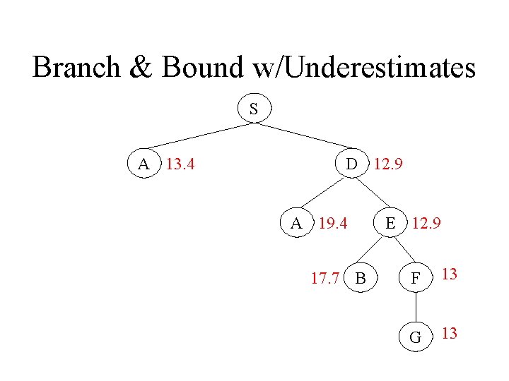
Branch & Bound w/Underestimates S A 13. 4 D 12. 9 A 19. 4 17. 7 B E 12. 9 F 13 G 13

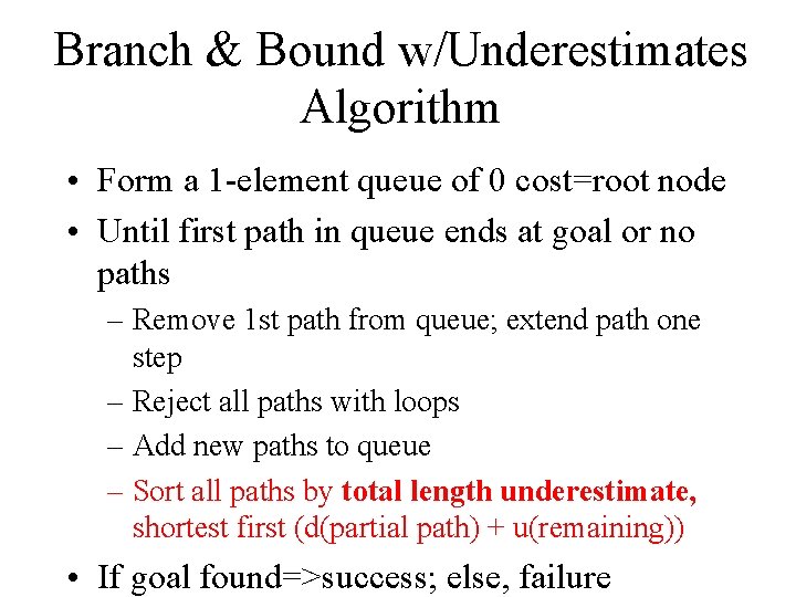
Branch & Bound w/Underestimates Algorithm • Form a 1 -element queue of 0 cost=root node • Until first path in queue ends at goal or no paths – Remove 1 st path from queue; extend path one step – Reject all paths with loops – Add new paths to queue – Sort all paths by total length underestimate, shortest first (d(partial path) + u(remaining)) • If goal found=>success; else, failure

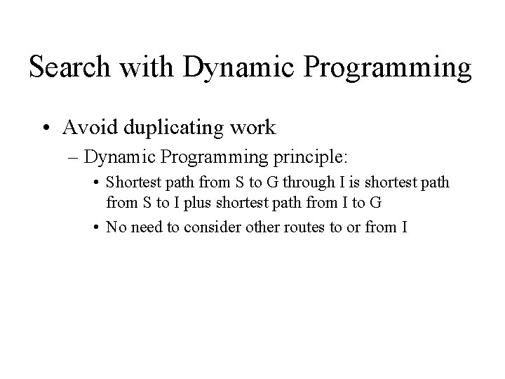
Search with Dynamic Programming • Avoid duplicating work – Dynamic Programming principle: • Shortest path from S to G through I is shortest path from S to I plus shortest path from I to G • No need to consider other routes to or from I

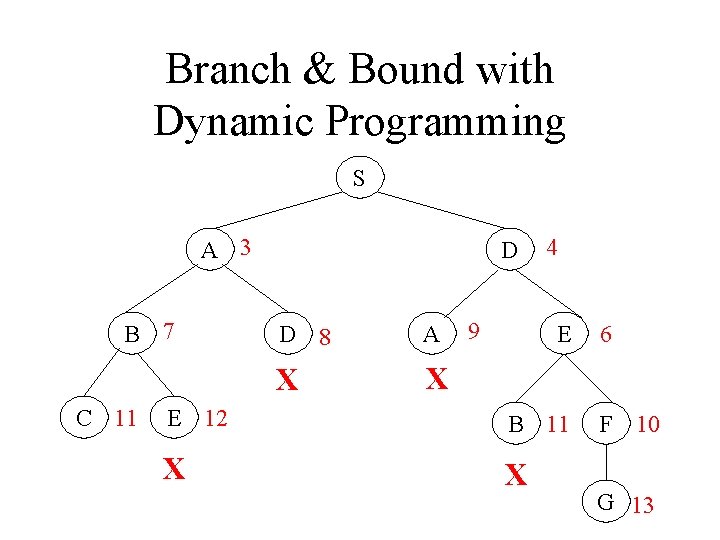
Branch & Bound with Dynamic Programming S A 3 B 7 C 11 D D 8 A X X 9 4 E E 12 B 11 X X 6 F 10 G 13

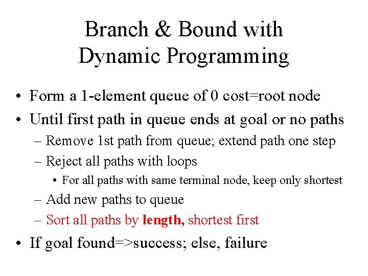
Branch & Bound with Dynamic Programming • Form a 1 -element queue of 0 cost=root node • Until first path in queue ends at goal or no paths – Remove 1 st path from queue; extend path one step – Reject all paths with loops • For all paths with same terminal node, keep only shortest – Add new paths to queue – Sort all paths by length, shortest first • If goal found=>success; else, failure

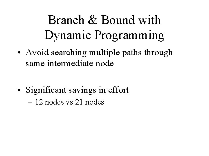
Branch & Bound with Dynamic Programming • Avoid searching multiple paths through same intermediate node • Significant savings in effort – 12 nodes vs 21 nodes

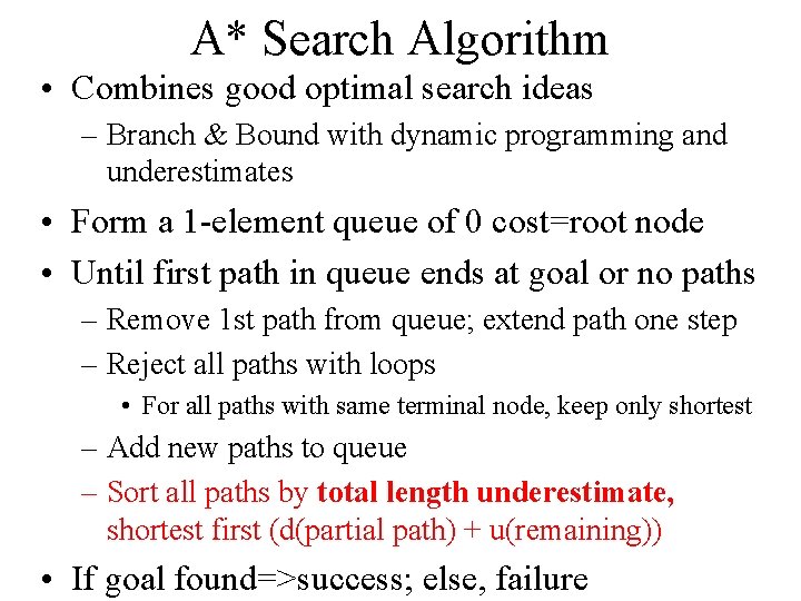
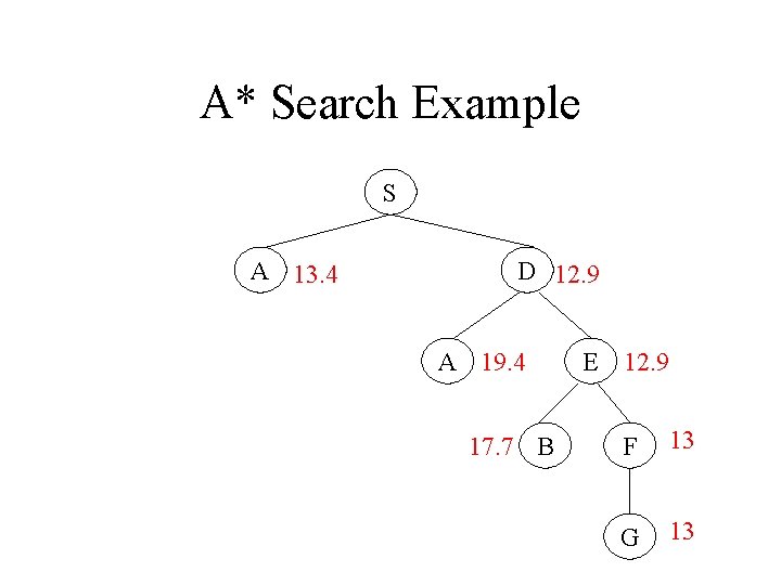
A* Search Algorithm • Combines good optimal search ideas – Branch & Bound with dynamic programming and underestimates • Form a 1 -element queue of 0 cost=root node • Until first path in queue ends at goal or no paths – Remove 1 st path from queue; extend path one step – Reject all paths with loops • For all paths with same terminal node, keep only shortest – Add new paths to queue – Sort all paths by total length underestimate, shortest first (d(partial path) + u(remaining)) • If goal found=>success; else, failure

A* Search Example S A 13. 4 D 12. 9 A 19. 4 17. 7 B E 12. 9 F 13 G 13

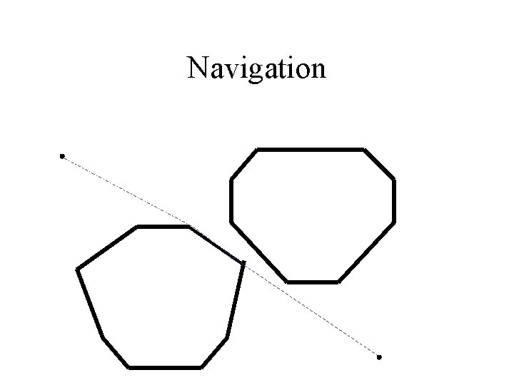
Navigation

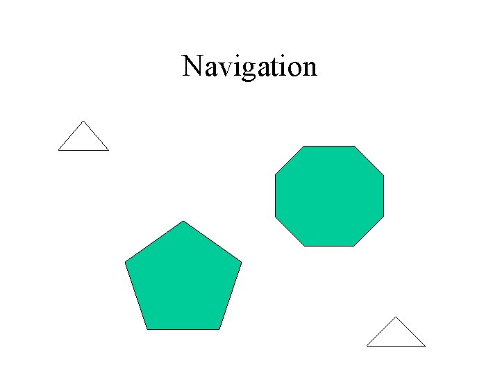
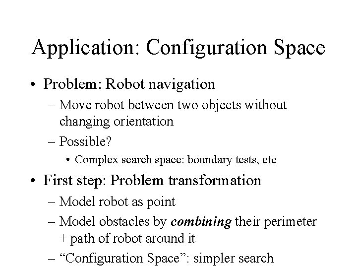
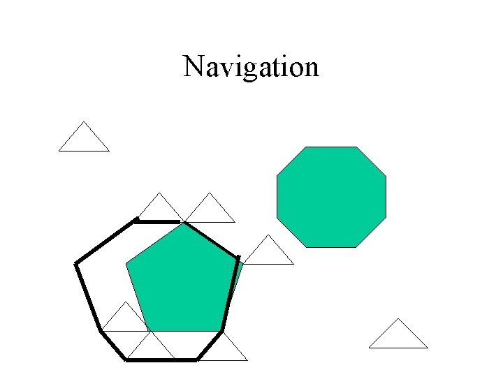
Application: Configuration Space • Problem: Robot navigation – Move robot between two objects without changing orientation – Possible? • Complex search space: boundary tests, etc • First step: Problem transformation – Model robot as point – Model obstacles by combining their perimeter + path of robot around it – “Configuration Space”: simpler search

Navigation

Navigation

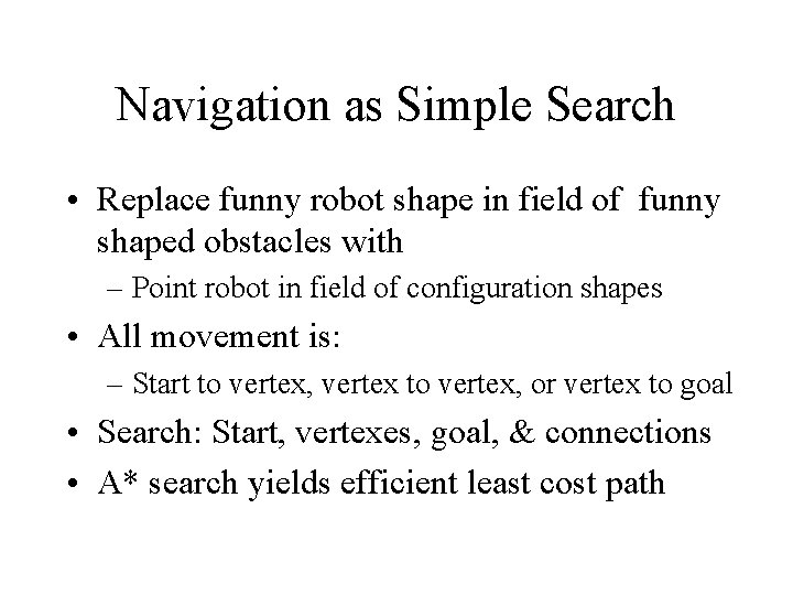
Navigation as Simple Search • Replace funny robot shape in field of funny shaped obstacles with – Point robot in field of configuration shapes • All movement is: – Start to vertex, vertex to vertex, or vertex to goal • Search: Start, vertexes, goal, & connections • A* search yields efficient least cost path

Summary • Optimal search: – Least cost solution with least work • British Museum procedure – Exhaustive search: report best • Branch & Bound: – Rank options by length; stop when partials>complete – Rank options by underestimate of TOTAL length – Dynamic programming: avoid unnecessary work • A*: B&B + Dynamic Programming + Underest

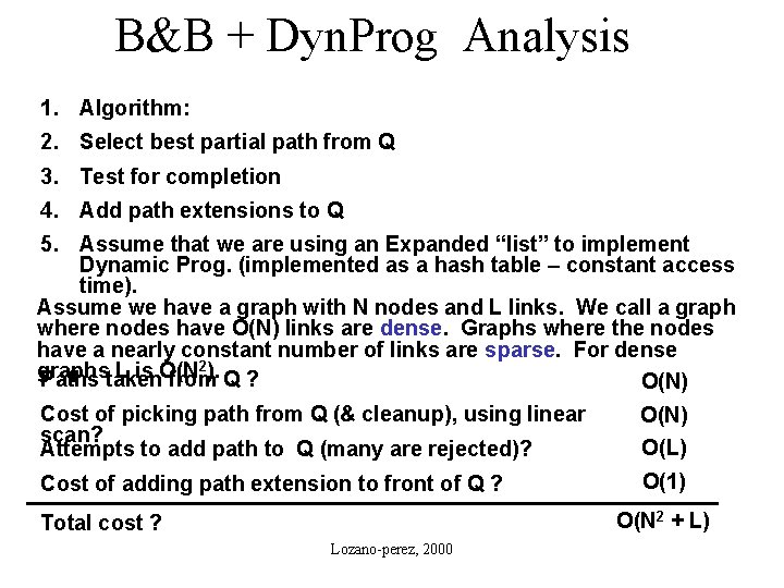
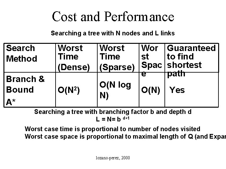
B&B + Dyn. Prog Analysis 1. Algorithm: 2. Select best partial path from Q 3. Test for completion 4. Add path extensions to Q 5. Assume that we are using an Expanded “list” to implement Dynamic Prog. (implemented as a hash table – constant access time). Assume we have a graph with N nodes and L links. We call a graph where nodes have O(N) links are dense. Graphs where the nodes have a nearly constant number of links are sparse. For dense 2 graphs L is O(N Paths taken from). Q ? O(N) Cost of picking path from Q (& cleanup), using linear O(N) scan? O(L) Attempts to add path to Q (many are rejected)? O(1) Cost of adding path extension to front of Q ? O(N 2 + L) Total cost ? Lozano-perez, 2000

Cost and Performance Searching a tree with N nodes and L links Search Method Worst Time (Dense) Branch & Bound A* O(N 2) Worst Wor Guaranteed Time st to find (Sparse) Spac shortest e path O(N log O(N) Yes N) Searching a tree with branching factor b and depth d L = N= b d+1 Worst case time is proportional to number of nodes visited Worst case space is proportional to maximal length of Q (and Expan lozano-perez, 2000