RFQ Development for FETS Simon Jolly Imperial College

RFQ Development for FETS Simon Jolly Imperial College 7 th January 2010

FETS RFQ Development • FETS will utilise a 4 m-long, 324 MHz four-vane RFQ channel, consisting of four resonantly coupled sections. • RFQ focuses beam from LEBT and accelerates it to 3 Me. V, ready for Chopper/MEBT. • 4 -vane cold model showed agreement between CST simulations and bulk RF properties. • Previous beam dynamics simulations, based on field maps produced with a field approximation code, provide a baseline for the new design. • Novel design method currently under development to combine CAD and electromagnetic modeling with beam dynamics simulations in GPT. 7/1/10 Simon Jolly, Imperial College 2

FETS Integrated RFQ Design • Would like to have a method of designing RFQ where all steps are integrated: – Engineering design. – EM modelling. – Beam dynamics simulations. • Integrating design steps allows us to characterise effects of: – Fringe fields and higher order modes. – Particular CNC machining techniques and options on beam dynamics. 7/1/10 Simon Jolly, Imperial College 3

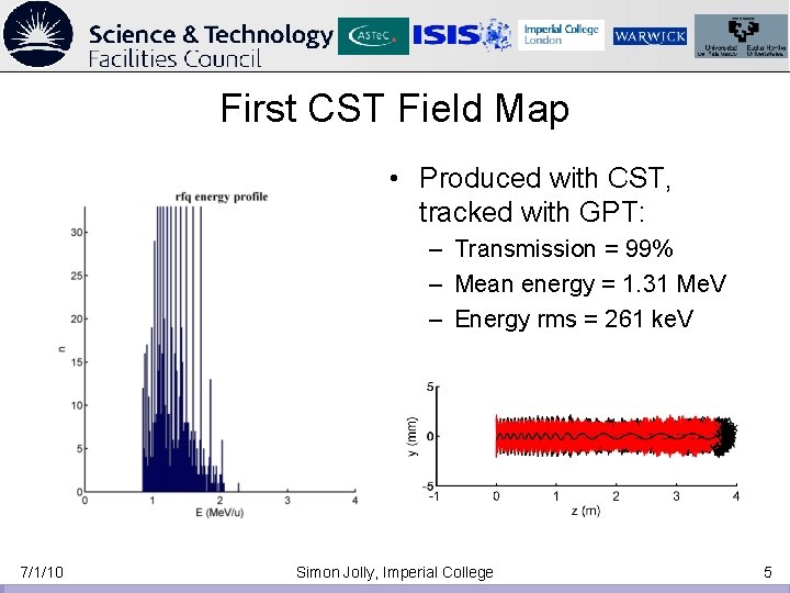
CST Mesh Density • A lot of effort on optimising meshing in CST. • Need a field map that gives transmission results similar to RFQSIM. • Important to quantify whether we can model Electrostatic field of vanes with enough accuracy in CST to measure beam dynamics. • Non-trivial: modelling 30 mm x 4 m volume with micron accuracy. • Changes in beam dynamics MUST be unaffected by coarseness of CST field meshing so we can compare to optimised field. 7/1/10 Simon Jolly, Imperial College 4

First CST Field Map • Produced with CST, tracked with GPT: – Transmission = 99% – Mean energy = 1. 31 Me. V – Energy rms = 261 ke. V 7/1/10 Simon Jolly, Imperial College 5

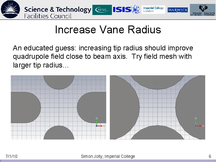
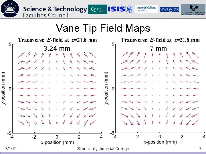
Increase Vane Radius An educated guess: increasing tip radius should improve quadrupole field close to beam axis. Try field mesh with larger tip radius… 7/1/10 Simon Jolly, Imperial College 6

Vane Tip Field Maps 3. 24 mm 7/1/10 7 mm Simon Jolly, Imperial College 7

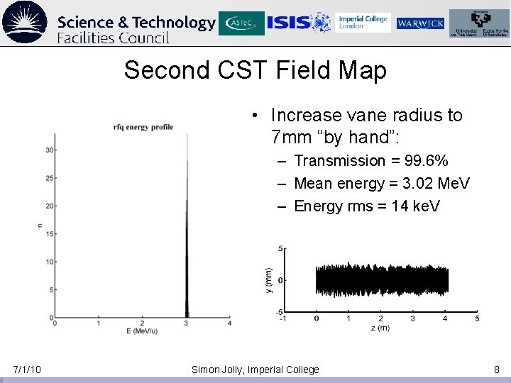
Second CST Field Map • Increase vane radius to 7 mm “by hand”: – Transmission = 99. 6% – Mean energy = 3. 02 Me. V – Energy rms = 14 ke. V 7/1/10 Simon Jolly, Imperial College 8

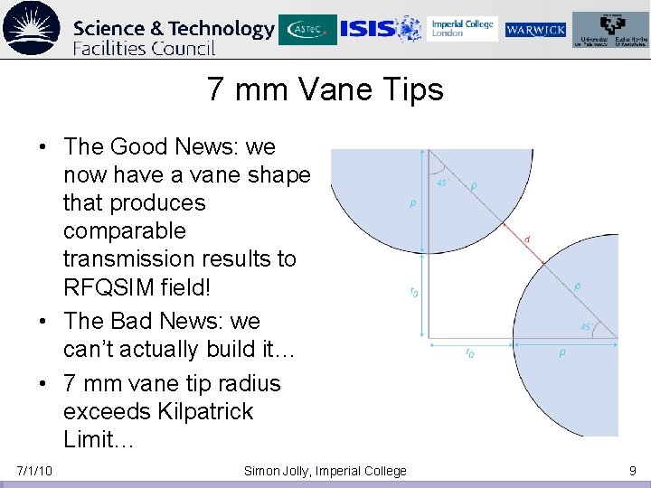
7 mm Vane Tips • The Good News: we now have a vane shape that produces comparable transmission results to RFQSIM field! • The Bad News: we can’t actually build it… • 7 mm vane tip radius exceeds Kilpatrick Limit… 7/1/10 Simon Jolly, Imperial College 9

22/4/09 State Of Play (Previous UKNF) • CAD modelling process now pretty mature: can model vane, rod and “vod” with parameter adjustment on-the-fly (everything except no. of cells). • Models import into CST and output to GPT: beam dynamics simulations well understood. • Definite issues in CST modelling: – We think we see “plateau” at 4, 100 points and 0. 5 mm point spacing of output file. – Clear discrepancies with Alan’s field map: good transmission and energy with r = 7 mm vane, r = 3. 2 mm rod but NOT r = 3. 2 mm vane! It should match… • Are the discrepancies real or down to faulty method? • Need to ensure we’re not re-inventing the wheel: RFQ’s have been designed before without this process. • Need to ensure CAM systems will understand our CAD models so we can manufacture what we’re designing (this is the point…). 7/1/10 Simon Jolly, Imperial College 10

Corrected Input Values • Couldn’t understand why increasing the radius of curvature made the results closer to Alan’s field map. • The solution: – Inconsistencies in the units of the RFQSIM input file. – Reported radius was incorrect, so RFQSIM actually modelling a larger radius. • Reran RFQSIM with corrected values to get new modulation parameters. 7/1/10 Simon Jolly, Imperial College 11

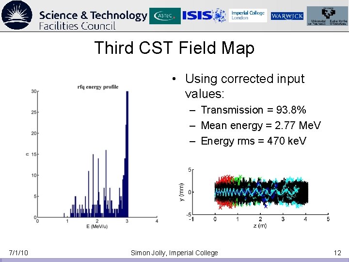
Third CST Field Map • Using corrected input values: – Transmission = 93. 8% – Mean energy = 2. 77 Me. V – Energy rms = 470 ke. V 7/1/10 Simon Jolly, Imperial College 12

Incoherent Acceleration • Better results: – Some particles accelerated to the full 3 Me. V. – Still not achieving coherent acceleration, even with new modulation parameters. – This result published at PAC’ 09. • Most obvious way to improve results is to increase mesh density: – Prior studies with 7 mm vanes showed current mesh density was sufficient. – Smaller radius of curvature (3. 24 mm) needs tighter mesh to model vane tip region. – CST at computational limit: split RFQ into 5 sections and mesh separately. 7/1/10 Simon Jolly, Imperial College 13

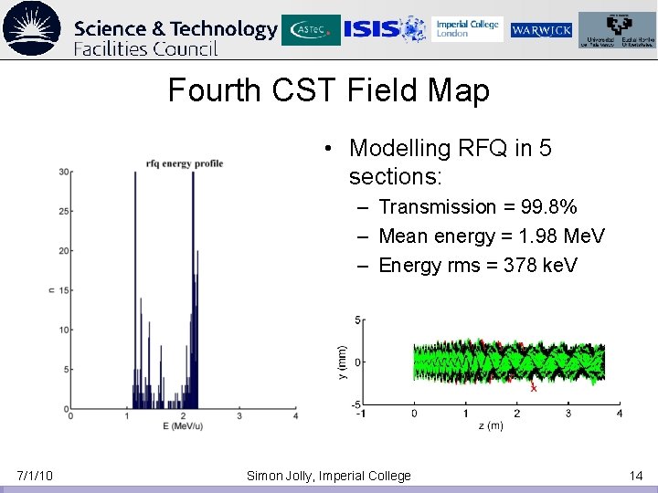
Fourth CST Field Map • Modelling RFQ in 5 sections: – Transmission = 99. 8% – Mean energy = 1. 98 Me. V – Energy rms = 378 ke. V 7/1/10 Simon Jolly, Imperial College 14

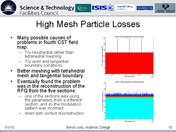
High Mesh Particle Losses • Many possible causes of problems in fourth CST field map: – Try hexahedral rather than tetrahedral meshing. – Try open and tangential boundary conditions. • Better meshing with tetrahedral mesh and tangential boundary. • Eventually found the problem was in the reconstruction of the RFQ from the five sections: – one of the sections was using the parameters from a different section, and so the modulation pattern was incorrect. – reran with correct reconstruction 7/1/10 Simon Jolly, Imperial College 15

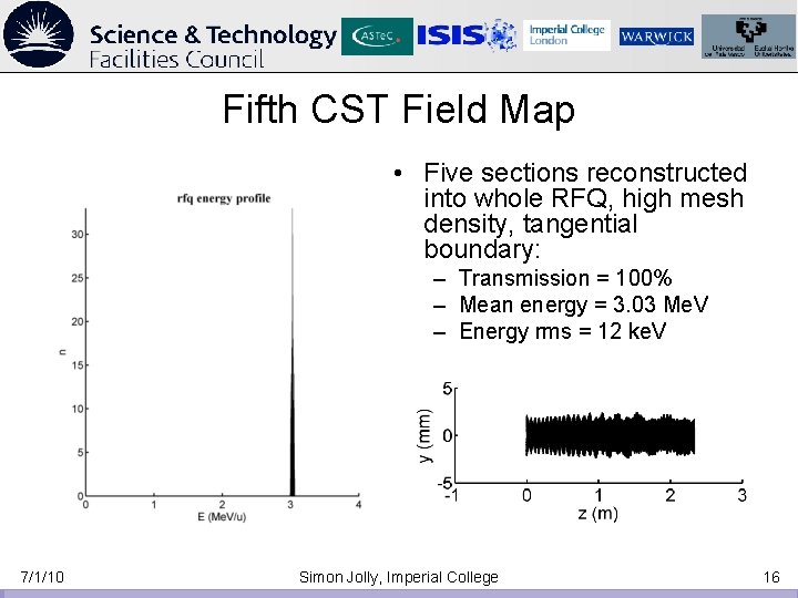
Fifth CST Field Map • Five sections reconstructed into whole RFQ, high mesh density, tangential boundary: – Transmission = 100% – Mean energy = 3. 03 Me. V – Energy rms = 12 ke. V 7/1/10 Simon Jolly, Imperial College 16

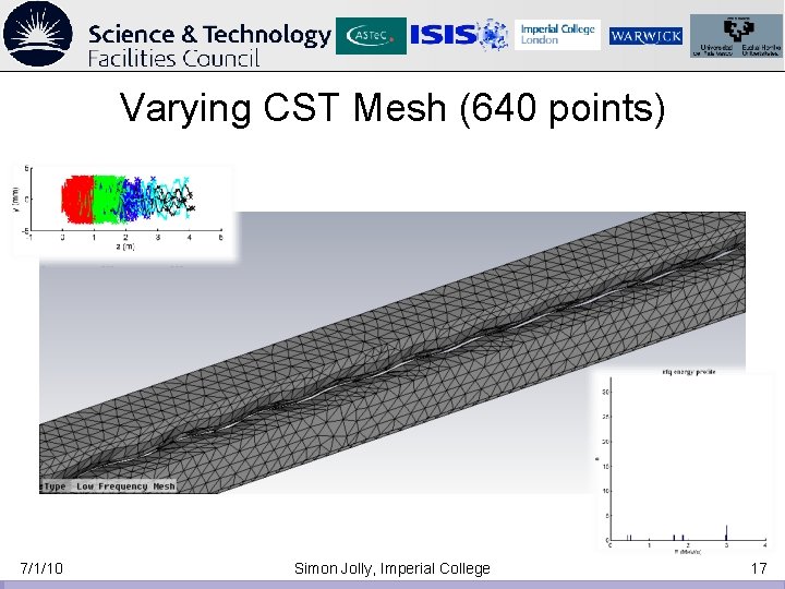
Varying CST Mesh (640 points) 7/1/10 Simon Jolly, Imperial College 17

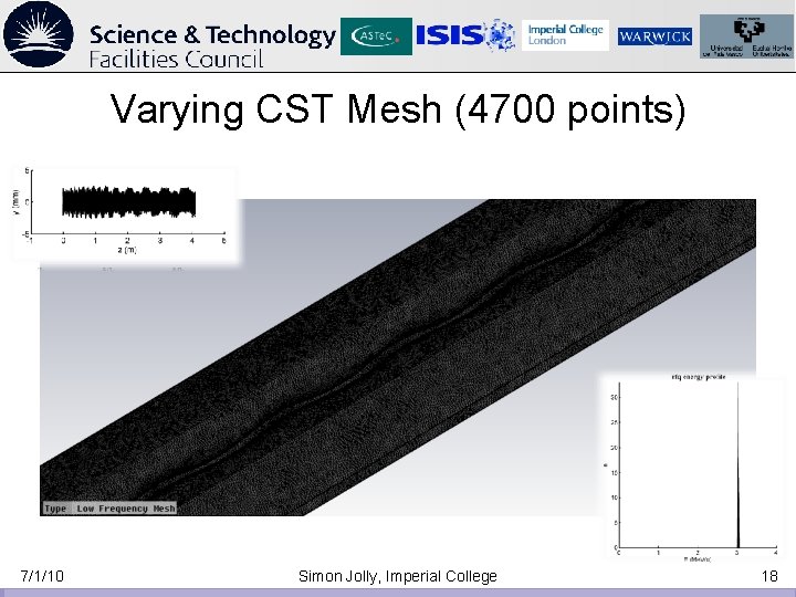
Varying CST Mesh (4700 points) 7/1/10 Simon Jolly, Imperial College 18

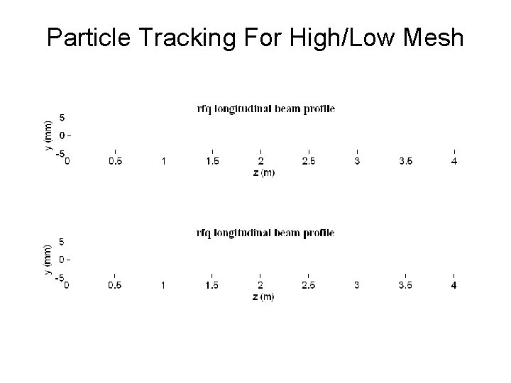
Particle Tracking For High/Low Mesh

Conclusions • Finally seeing match between RFQSIM optimised field map and CST field map from CAD modelling. • Each step has required a lot of effort for small progress, but that progress has proved extremely valuable. • Advantages of this process already starting to become apparent: for example, very easy to modify CAD model based on thermal/stress simulations (Scott Lawrie) and measure effect on beam dynamics. • Next steps: – Output CAD model to Comsol, repeat process from CST to produce more easily adaptable field map (tighter integration with Inventor and Matlab). – Compare CST coarse, fine, Comsol and RFQSIM field maps point-by-point to determine whether discrepancies are a result of poor field mapping or more accurate modelling of vane tips. 7/1/10 Simon Jolly, Imperial College 20

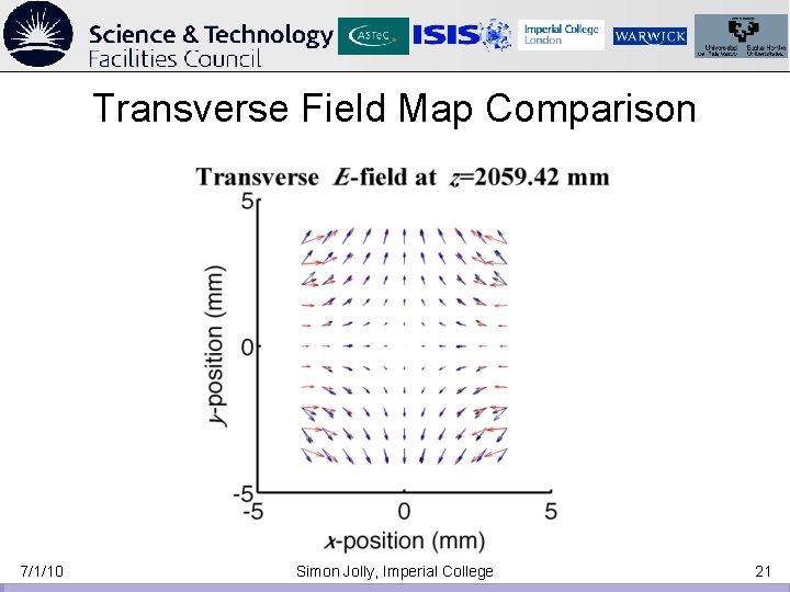
Transverse Field Map Comparison 7/1/10 Simon Jolly, Imperial College 21

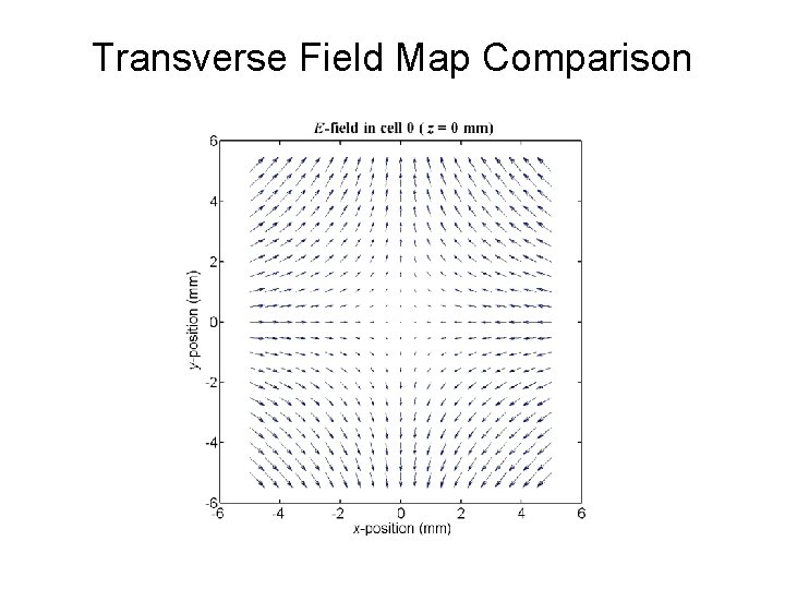
Transverse Field Map Comparison

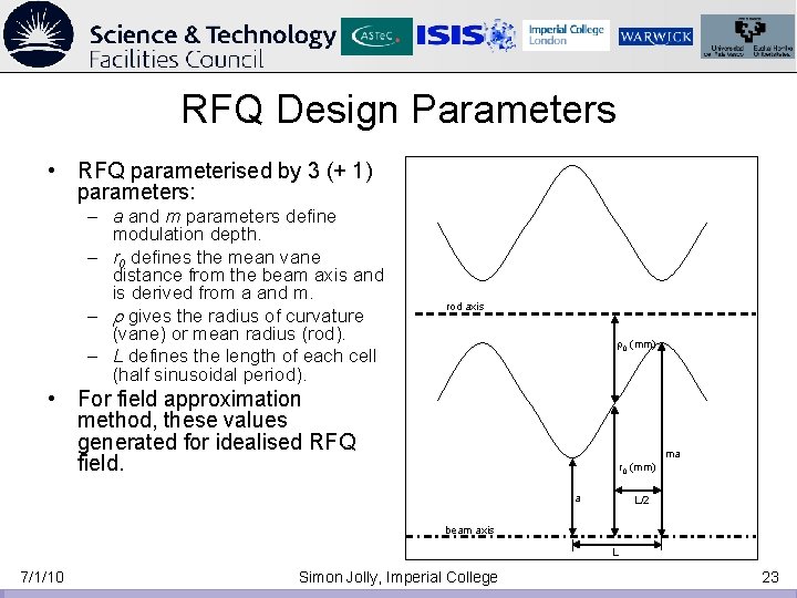
RFQ Design Parameters • RFQ parameterised by 3 (+ 1) parameters: – a and m parameters define modulation depth. – r 0 defines the mean vane distance from the beam axis and is derived from a and m. – r gives the radius of curvature (vane) or mean radius (rod). – L defines the length of each cell (half sinusoidal period). rod axis r 0 (mm) • For field approximation method, these values generated for idealised RFQ field. ma r 0 (mm) a L/2 beam axis L 7/1/10 Simon Jolly, Imperial College 23

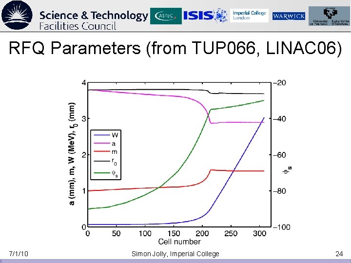
RFQ Parameters (from TUP 066, LINAC 06) 7/1/10 Simon Jolly, Imperial College 24

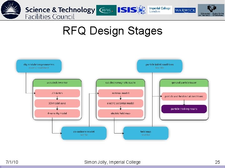
RFQ Design Stages 7/1/10 Simon Jolly, Imperial College 25

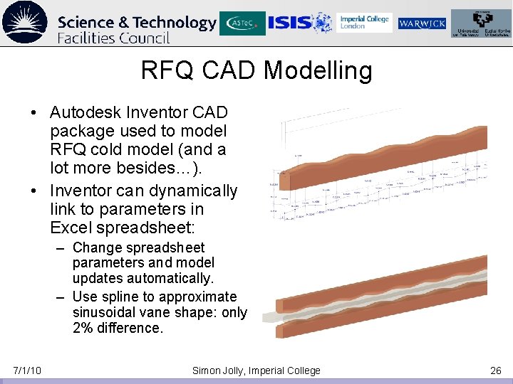
RFQ CAD Modelling • Autodesk Inventor CAD package used to model RFQ cold model (and a lot more besides…). • Inventor can dynamically link to parameters in Excel spreadsheet: – Change spreadsheet parameters and model updates automatically. – Use spline to approximate sinusoidal vane shape: only 2% difference. 7/1/10 Simon Jolly, Imperial College 26

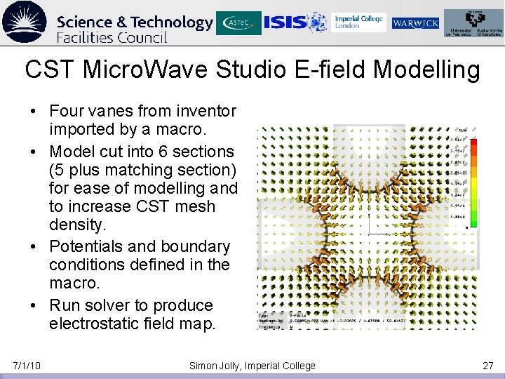
CST Micro. Wave Studio E-field Modelling • Four vanes from inventor imported by a macro. • Model cut into 6 sections (5 plus matching section) for ease of modelling and to increase CST mesh density. • Potentials and boundary conditions defined in the macro. • Run solver to produce electrostatic field map. 7/1/10 Simon Jolly, Imperial College 27

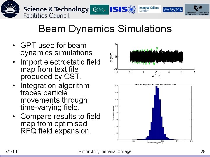
Beam Dynamics Simulations • GPT used for beam dynamics simulations. • Import electrostatic field map from text file produced by CST. • Integration algorithm traces particle movements through time-varying field. • Compare results to field map from optimised RFQ field expansion. 7/1/10 Simon Jolly, Imperial College 28