Raster Analysis MingChun Lee 1 Raster Analysis Performed

Raster Analysis Ming-Chun Lee 1

Raster Analysis Performed on cells and grids. Raster cells store data ◦ Nominal – land use ◦ Ordinal – street classification ◦ Interval/Ratio – temperature, elevation manipulations on cell values for a single raster layer or multiple layers. Perform analysis based on 2

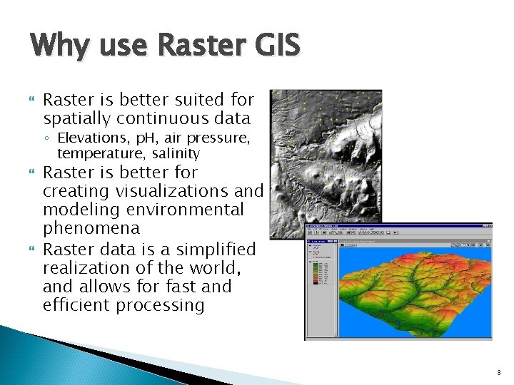
Why use Raster GIS Raster is better suited for spatially continuous data ◦ Elevations, p. H, air pressure, temperature, salinity Raster is better for creating visualizations and modeling environmental phenomena Raster data is a simplified realization of the world, and allows for fast and efficient processing 3

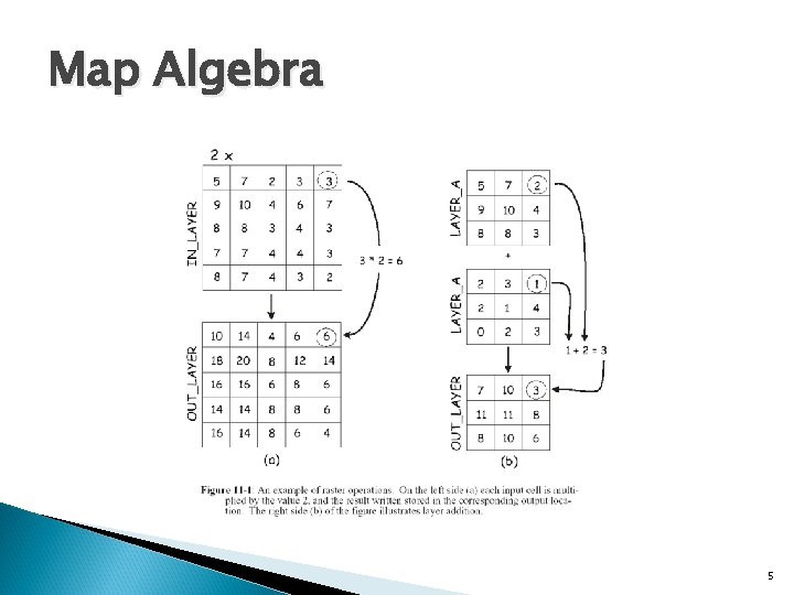
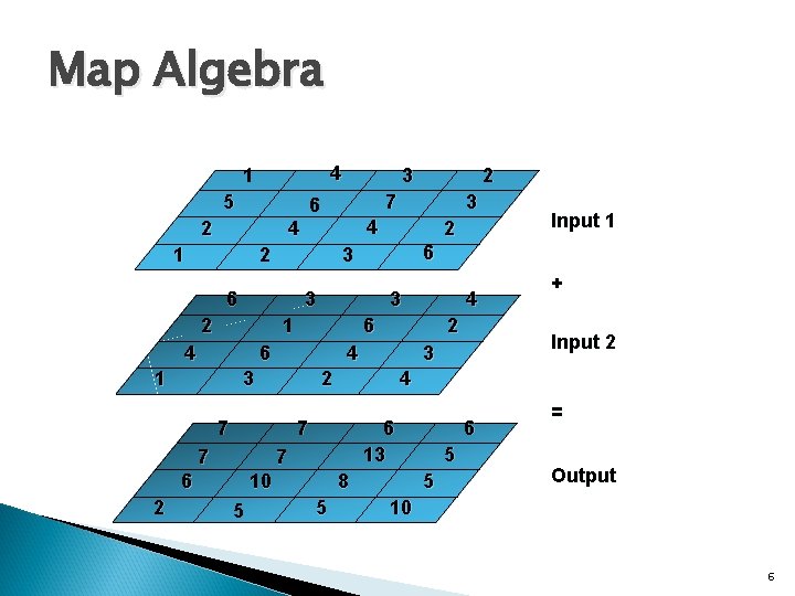
Map Algebra Cell by Cell combination of raster data layers using mathematical operations ◦ one layer ◦ multiple layers Each number represents a value at a raster cell location Simple operations can be applied to each number Raster layers may be combined through operations ◦ Addition, subtraction and multiplication 4

Map Algebra 5

Map Algebra 4 1 5 2 3 1 1 3 4 6 13 7 6 10 5 8 5 + Input 2 3 2 7 7 2 4 7 4 6 6 Input 1 6 3 4 2 3 6 2 3 4 4 1 2 7 6 2 2 3 6 5 5 = Output 10 6

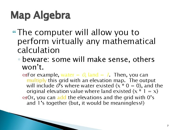
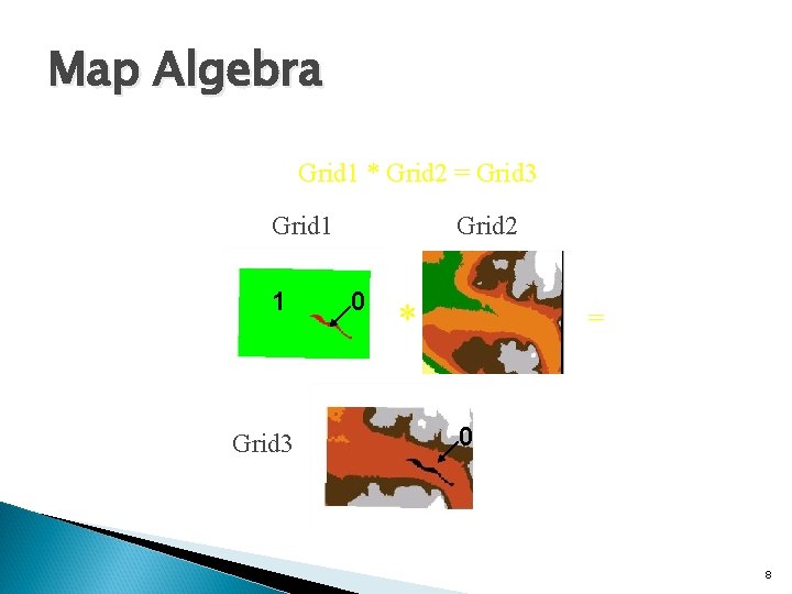
Map Algebra The computer will allow you to perform virtually any mathematical calculation ◦ beware: some will make sense, others won’t. For example, water = 0, land = 1. Then, you can multiply this grid with an elevation map. The output will include 0’s where water existed (x * 0 = 0), and the original elevation value where land existed (x * 1 = x) Or, you can add the elevations and the grid with 0’s and 1’s together (but, it would be meaningless!) 7

Map Algebra Grid 1 * Grid 2 = Grid 3 Grid 1 1 Grid 3 Grid 2 0 * = 0 8

Map Algebra Multiple grid themes share the same X, Y coordinate space A single output grid theme is the result of the multiple grids 9

Map Algebra Mathematical Operators: ◦ Arithmetic +, -, *, / ◦ Boolean AND, OR, NOT, XOR ◦ Relational =, <, >, ≤, ≥, <> ◦ Algebraic Functions Powers & Roots, Trigonometry, Logarithm 10

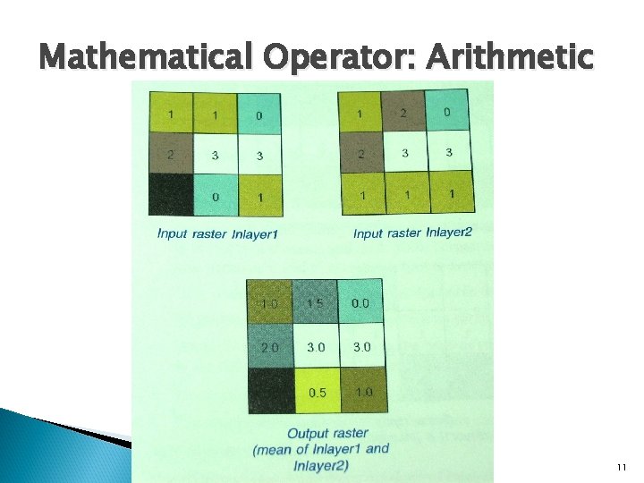
Mathematical Operator: Arithmetic 11

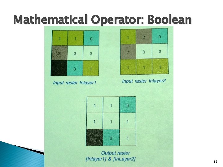
Mathematical Operator: Boolean 12

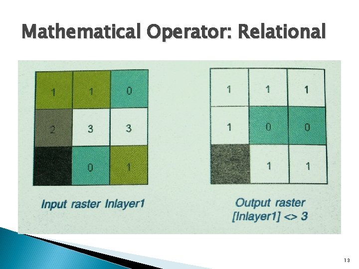
Mathematical Operator: Relational 13

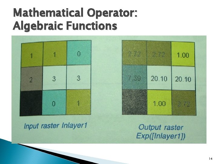
Mathematical Operator: Algebraic Functions 14

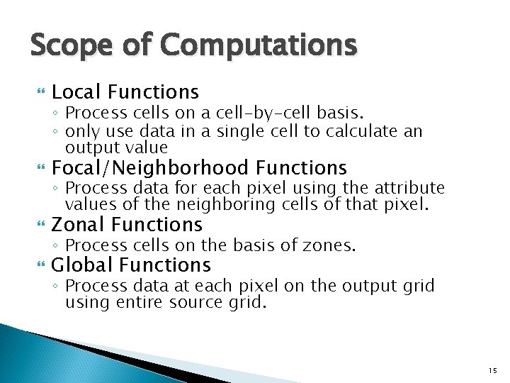
Scope of Computations Local Functions Focal/Neighborhood Functions Zonal Functions Global Functions ◦ Process cells on a cell-by-cell basis. ◦ only use data in a single cell to calculate an output value ◦ Process data for each pixel using the attribute values of the neighboring cells of that pixel. ◦ Process cells on the basis of zones. ◦ Process data at each pixel on the output grid using entire source grid. 15

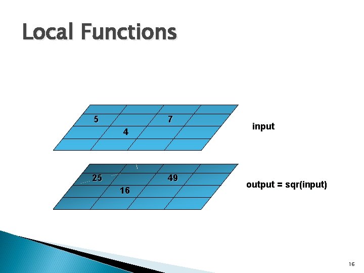
Local Functions 5 7 4 25 49 16 input output = sqr(input) 16

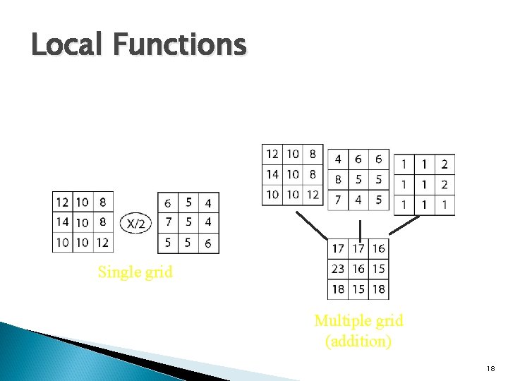
Local Functions Operations that modify a cell on a single grid ◦ Data type changes ◦ Arithmetic operations ◦ Converting one value to another according to a rule (Recode) Local operations on multiple layers ◦ Map algebra (Output = f(Input 1, Input 2, …) Functions may be mathematical or logical 17

Local Functions Single grid Multiple grid (addition) 18

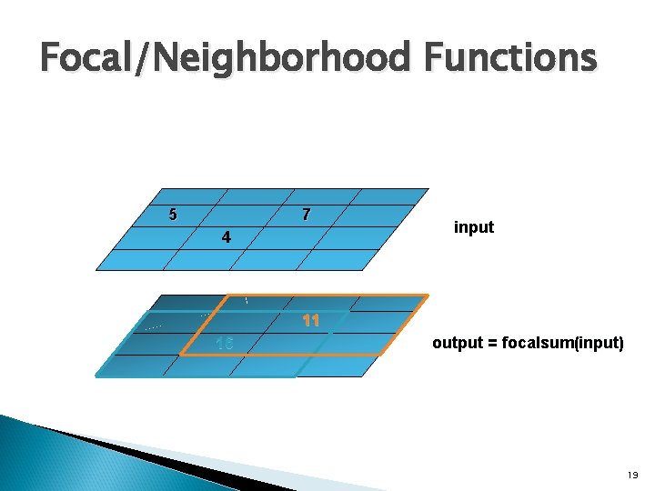
Focal/Neighborhood Functions 5 7 4 input 11 16 output = focalsum(input) 19

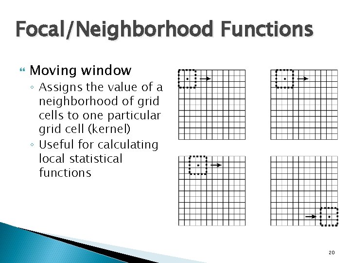
Focal/Neighborhood Functions Moving window ◦ Assigns the value of a neighborhood of grid cells to one particular grid cell (kernel) ◦ Useful for calculating local statistical functions 20

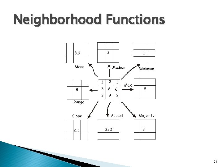
Neighborhood Functions 21

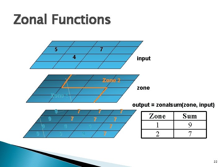
Zonal Functions 5 7 4 input Zone 2 zone Zone 1 output = zonalsum(zone, input) 9 7 9 9 7 7 Zone 1 2 Sum 9 7 22

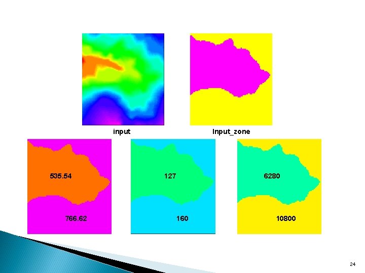
Zonal Functions Output value at each location depends on the values of all the input cells in an input value grid that shares the same input value zone Type of complex neighborhood function ◦ use complex neighborhoods or zones 23

input 535. 54 766. 62 Input_zone 127 6280 160 10800 24

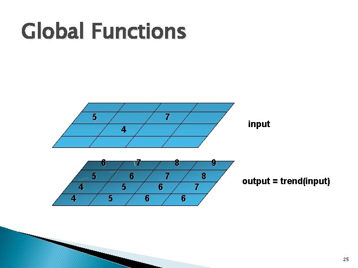
Global Functions 5 7 input 4 6 7 5 6 4 4 8 7 5 5 9 8 6 6 7 output = trend(input) 6 25

Global Functions Output value of each location is potentially a function of all the cells in the input grid ◦ e. g. distance functions, surfaces, interpolation, etc. 26

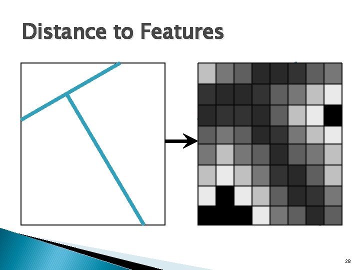
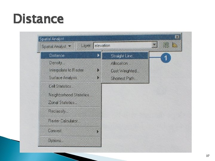
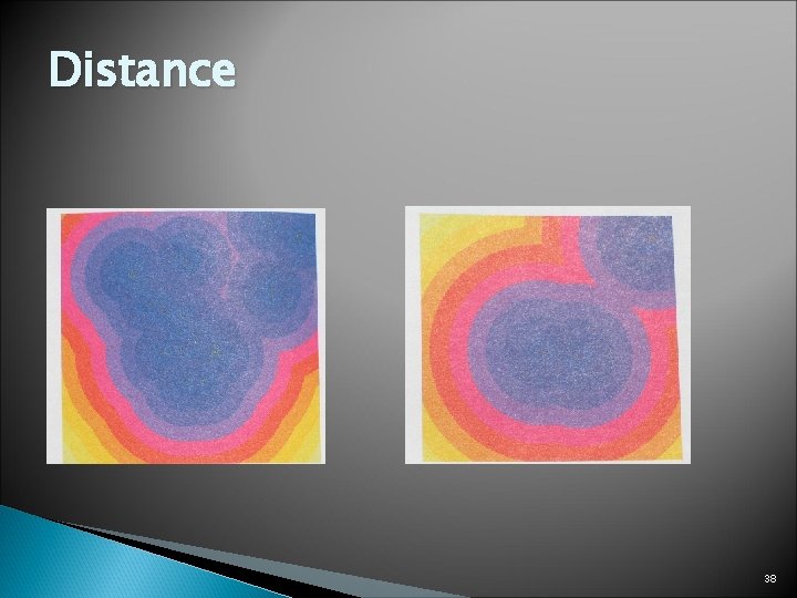
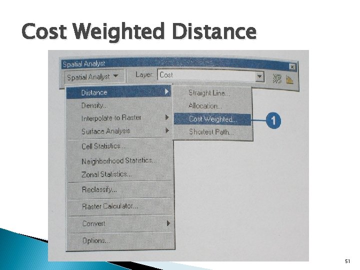
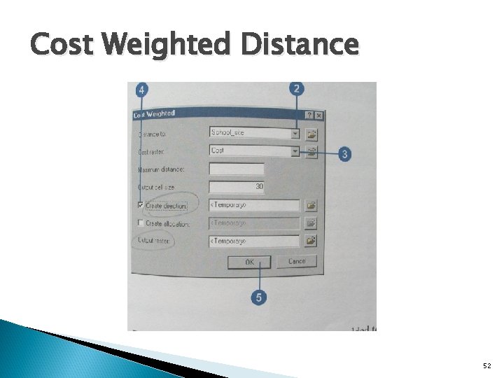
Distance to Features Cell value is the Distance from the Cell Center to the Nearest Feature(s) in a Specified Layer ◦ Physical distance– equivalent to buffers ◦ Cost distance Requires a cost grid as input Cost grid contains costs for unit distance Cost distance between two cells is the average of the two values multiplied by the distance between them Total cost is calculated to source cells. 27

Distance to Features 28

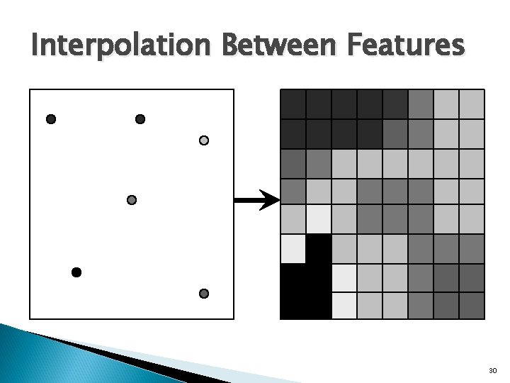
Interpolation Between Features Interpolation predicts values for cells in a raster from a limited number of sample data points. ◦ Elevation, rainfall, chemical concentration, noise level Average of Nearby Features’ Values, Weighted by Distance, Regardless of Density Example: Number of Bus Routes Serving a Neighborhood! 29

Interpolation Between Features 30

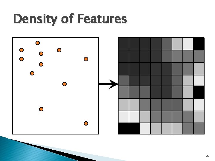
Density of Features Value Assigned Based on the Neighborhood Density of a Feature Can be Weighted on an Attribute Value ◦ Example: Estimate a Population Density Surface Using Census Tract Population ◦ Another Example – Bus Service Density 31

Density of Features 32

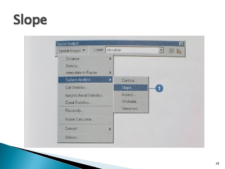
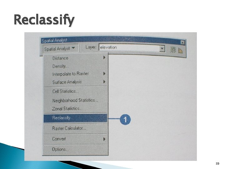
Spatial Analyst functions Find Distance Calculate Density Interpolate Surface Derive Slope, Aspect Create Contour Cell Statistics Summarize Zones Tabulate Areas Map Query, Calculator Neighborhood Statistics Reclassify 33

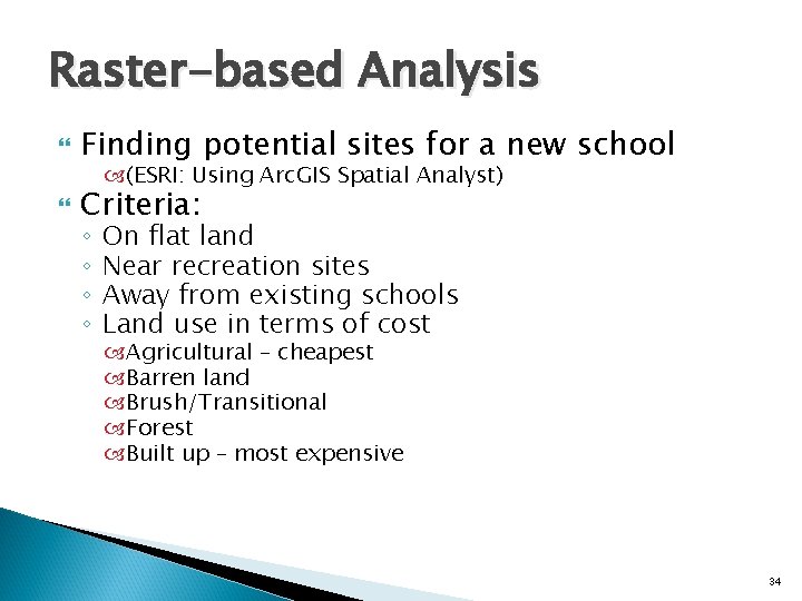
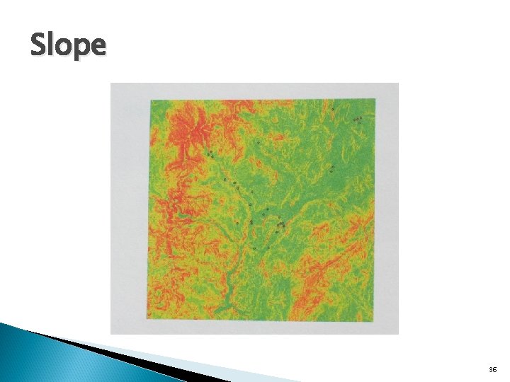
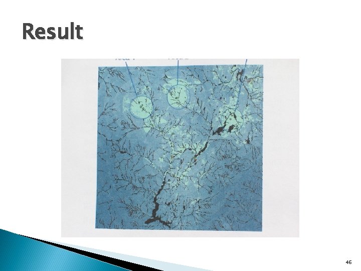
Raster-based Analysis Finding potential sites for a new school Criteria: (ESRI: Using Arc. GIS Spatial Analyst) ◦ ◦ On flat land Near recreation sites Away from existing schools Land use in terms of cost Agricultural – cheapest Barren land Brush/Transitional Forest Built up – most expensive 34

Slope 35

Slope 36

Distance 37

Distance 38

Reclassify 39

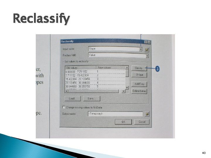
Reclassify 40

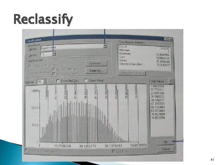
Reclassify 41

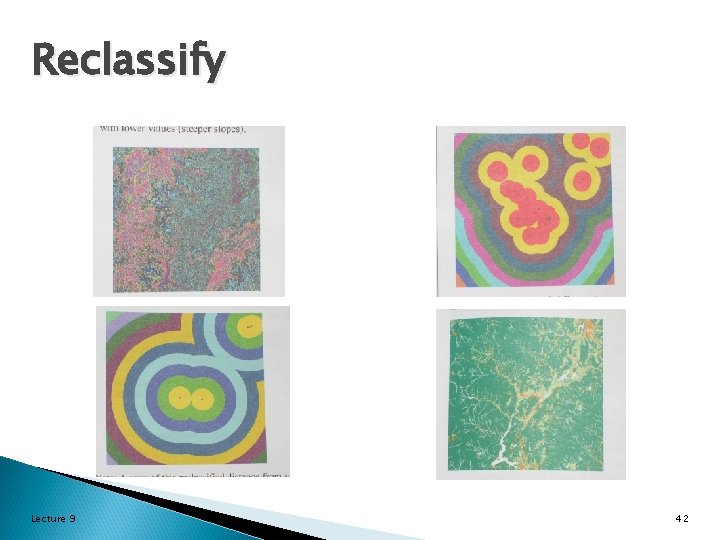
Reclassify Lecture 9 42

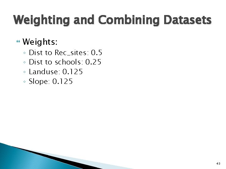
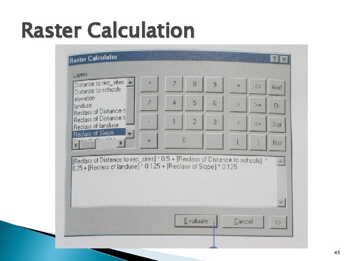
Weighting and Combining Datasets Weights: ◦ ◦ Dist to Rec_sites: 0. 5 Dist to schools: 0. 25 Landuse: 0. 125 Slope: 0. 125 43

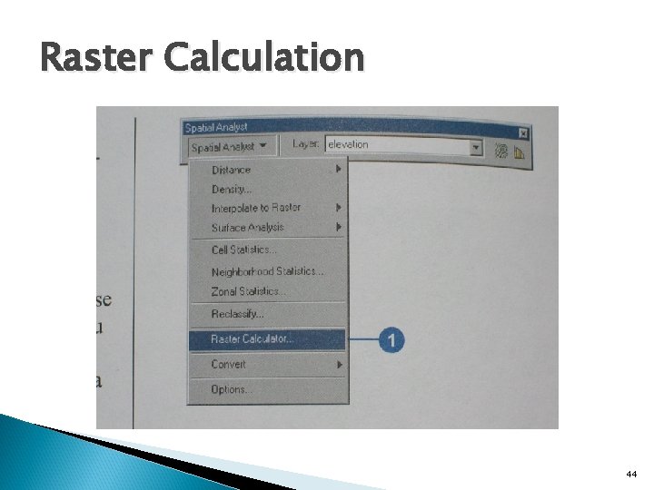
Raster Calculation 44

Raster Calculation 45

Result 46

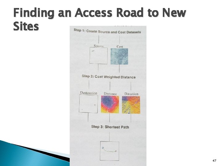
Finding an Access Road to New Sites 47

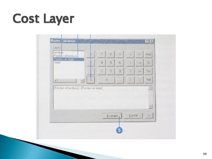
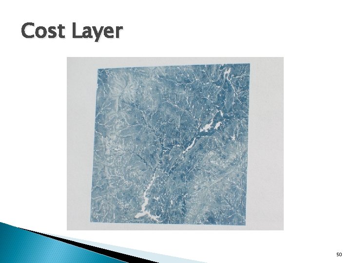
Cost Layer Slope: ◦ High values (10) to steeper slopes Land Use: ◦ ◦ ◦ Agricultural: 4 Brush/Transitional: 5 Barren land: 6 Forest: 8 Built up: 9 Water: 10 48

Cost Layer 49

Cost Layer 50

Cost Weighted Distance 51

Cost Weighted Distance 52

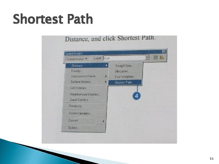
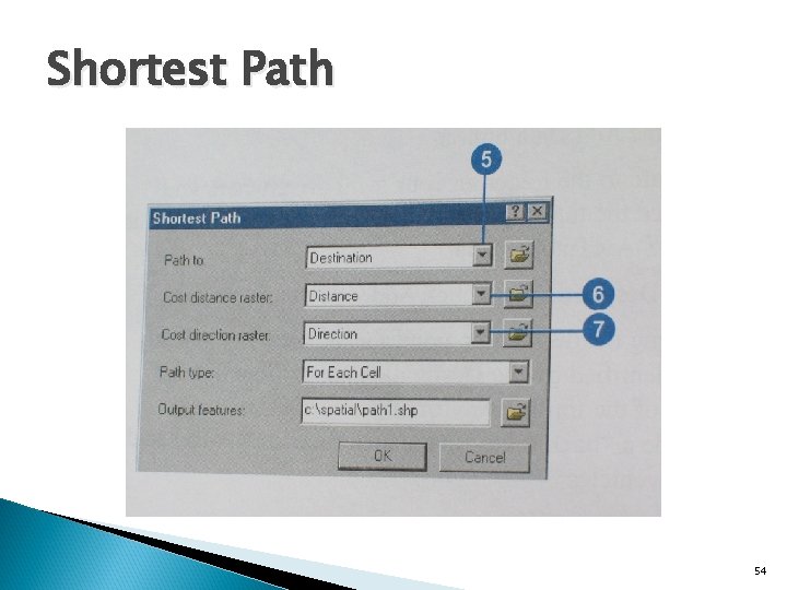
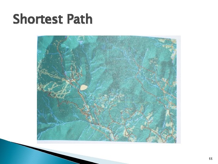
Shortest Path 53

Shortest Path 54

Shortest Path 55