Range Image Processing Archana Gupta What are range

Range Image Processing Archana Gupta

What are range images ? Range images are a special class of digital images where each pixel expresses the distance between a known reference frame and a visible point in the scene. They are also known as depth images.

Application of range images v Reverse engineering v Collaborative design v Inspection v Special effects, games & virtual worlds v Dissemination of museum artifacts v Medicine v Home shopping

Steps towards Range Image processing A. Data collection B. Data registration C. Data Modeling (geometry, texture and lighting

A. Data collection (a) (b)

Measurement principle Every pixel on the sensor samples the amount of modulated light reflected by objects in the scene. The phase shift between the emitted light and the returning signal determines the distance to the objects in the scene. This is illustrated by fig (a). A range image obtained from a scanner in fig (a) is a collection of points with regular spacing as shown in fig (b).

Problem with such data acquisition Some calibration has to be performed in order to get rid of the distortions and misalignments of the optical lens and sensor. As a result some data preprocessing is performed.

Preprocessing v. The uncertainty value generated by the sensor as a function of measured amplitude is used to filter out inaccurate data points. v A grid around the viewing range of sensor is decomposed into cells and each cell must contain a minimum no of data points to be considered occupied.

B. Data registration Registration involves having features in multiple scenes exactly match each other in location. In other words the key step here is to find a spatial transformation (linear in nature) such that a similarity metric between two or more images taken at different times and from different sensors or different viewpoints, achieves its maximum.

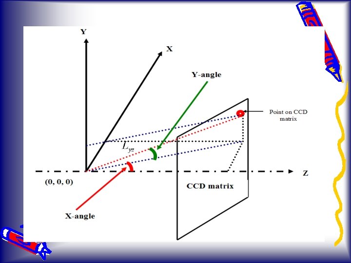
C. Data Modeling (geometry, texture and lighting) Surface Reconstruction v Size of CCD matrix 124 X 160 v Translate x and y so that CCD center aligns with origin of the coordinate system

Surface reconstruction cont… Finding angles

Surface reconstruction cont… Finding the real points

Mesh creation & simplification

v The faces are found and the mesh is created using the patch command in matlab. v The mesh is then simplified. There are many mesh simplification software available online. I made use of QSlim.

Mesh simplification algorithms v Vertex clustering: spatially partitions vertices and unifies vertices in same cluster. v Vertex decimation: selects unimportant vertices (based on local shape heuristics), remove them and retriangulate resulting holes. v Iterative Edge contraction: ranks edges and collapses one with least resulting error.

QSlim details QSlim uses an algorithm based on iterative edge contraction and quadric error metrics.

Quadric Error metrics v Each vertex has (conceptual) set of planes. v Vertex error = sum of squared distances to planes. v Combine sets when contracting vertex pair.

Measuring error with Quadrics

Measuring error with Quadrics cont. .

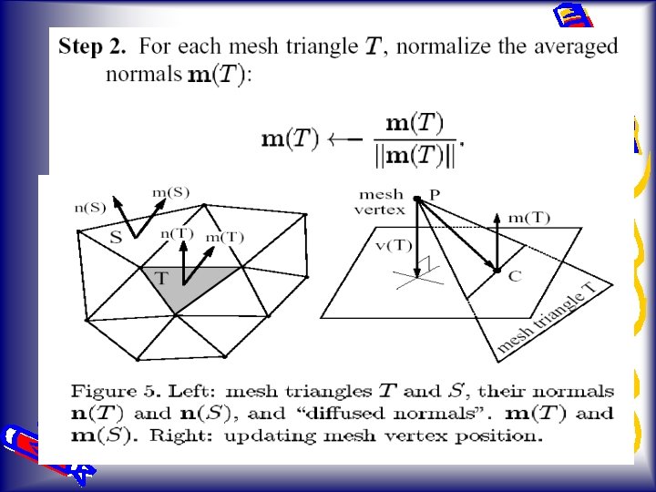
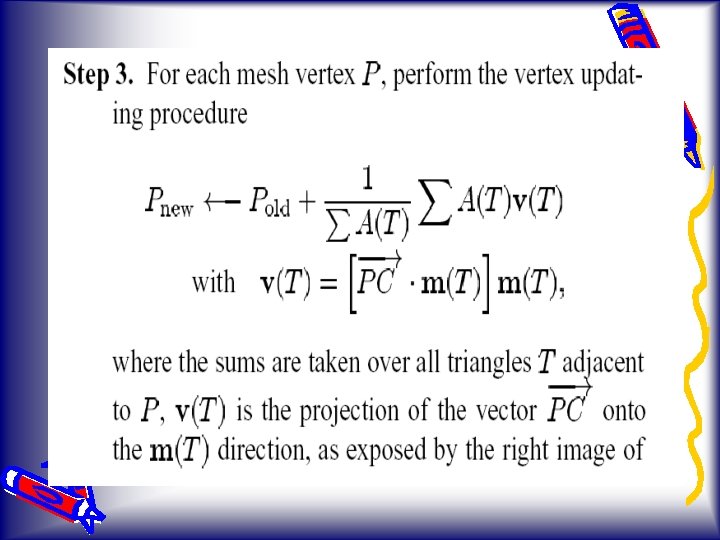
Mesh smoothing via mean filtering

Results

Initial Image

Image after filtering

3 D Cloud of image

3 D mesh

Mesh with 10000 faces

Mesh with 800 faces

Mesh with 500 faces

Mesh after mean smoothing 4 iterations

Mesh after mean smoothing 10 iterations

Conclusions • The mesh produced after converting image coordinates to real world coordinates is quite impressive. • The Qslim software works very well in simplifying the mesh to the number of triangle faces required by the user. • Finally the Mean filter for averaging face normals algorithm seems to do a good job at defining the ball but distorts the wall edges.

References v Thanks to Dr Latecki for his invaluable guidance v http: //www. csem. ch/detailed/pdf/p_531_SR 2_Preliminary-0355. pdf v http: //asl. epfl. ch/asl. Internal. Web/ASL/publicatio ns/uploaded. Files/2004 iros_weingarten. pdf v Introductory Techniques for 3 -D Computer Vision by Emanuele Trucco and Alessandro Verri v http: //graphics. uiuc. edu/~garland/software/qs lim. html v http: //www. u-aizu. ac. jp/labs/swsm/Yagou/gmp 02 yob. pdf