Radiation at particle accelerators Radiation Protection Radiation Protection

Radiation at particle accelerators Radiation Protection

Radiation Protection • Protecting people, workers and the environment • Radioactive waste management • Accelerators • Characterization and Services (e. g. transport, radioanalytical lab)

Radioactive decay Types of radioactivity can be differentiated as following: • α-Decay: An α- particle (a helium-nucleus) is emitted. • In this process the mass number decreases by four. • β-Decay: A neutron becomes a proton, which results in the emittion of a β-particle (an electron) and an anti-neutrino. • γ-Radiation: A photon is emitted by an unstable nucleus, resulting inγ-Radiation (part of electromagnetic spectrum).

Our projects: • Monte-Carlo-principles • Interaction of ionizing radiation with matter • Gamma spectroscopy • Particle camera • Simulations

Monte-Carlo-Principles • The Monte-Carlo-Principle is a mathematical method, with which problems can be solved, that are too complicated to calculate them otherwise. • The two main components are: - Random numbers - A similar problem

Monte-Carlo-Simulations

Simulations are used to test e. g. : • shielding designs • accelerator designs • dosimetry and radioprotection

• The software used to run the simulations is FLUKA (FLUktuierende Kascade) • Necessary parameters for simulations: • • • Particle type Starting point Direction Energy Geometry

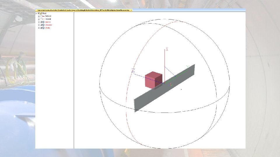
Overview of our simulations • Simulation of particles originating from typical radioactivity decays, including the simulation of the effect a shielding material placed in front of the source • a) Alpha particles • b) Beta particles • c) Gamma particles Simulation of a high-energy particle impacting on a copper cylinder (target) • a) No magnetic field surrounding the target • b) Strong magnetic field surrounding the target

Beta-Strahlung (1 Ge. V), shielded by 1 mm aluminium

Beta-Strahlung (1 Ge. V), shielded by 2 mm aluminium

e. V G 0 to Pro 5 ith w n Copper target starting at (0, 0, 0) with a length of 20 cm and a radius of 3 cm, oriented along z axis.

Gamma specs- Gamma ray absorption in matter

The High Purity Germanium Detector (HPGE) With the detector one can measure the radiation emitted by a source, as well as the absorption rate of different materials. • The detector is a germanium detector. Germanium is a semiconductor, which requires cryogenic temperatures to operate (77 Kelvin) • The detector is cooled liquid nitrogen, in order for it work.

Measurements Step 1: Open the detector and place the Cobalt 60 in the centre of the plate. Now the detector measures the radiation emitted by the source of radiation, which in this case is Cobalt 60.

Step 2: Close the door of the detector shielding and start running the measurements. In order to achieve a statistical certainty of less than 1%, the detector has to measure at least 20000 counts per second- meaning it has to detect at least 200000 particles.

Step 3: Once the detector has reached 20000 cps, stop the machine and save the file. Step 4: Open the detector shielding and place one screen of a metal between the source and the detector. Repeat the measurements and save the new file. Continue adding more screens of metals.

Number of Screen Material 0 1 2 3 4 5 6 7 8 9 0 1 2 3 4 5 6 0 1 2 3 4 1 Steel Steel Steel Brass Brass Aluminium Lead Paper Thickness mm 0 1. 5 3 4. 5 6 7. 5 9 10. 5 12 13. 5 0 0. 5 1 1. 5 2 2. 5 3 0 1 6 0 2. 2 4. 4 6. 6 8. 8 11 1173 k. Ev 1332 ke. V time counts cps counts time cps s 23467. 83 117. 5 199. 7262 21118. 49 117. 5 179. 7318 23314. 72 124. 7611 186. 9 20836. 99 124. 7611 167. 0151 22896. 14 131. 07 174. 7 20693. 99 131. 07 157. 885 22835. 58 138. 71 164. 6 20663. 09 138. 71 148. 9661 22424. 07 146. 72 152. 8 20398. 54 146. 72 139. 0304 22217. 87 153. 95 144. 3 20209. 73 153. 95 131. 2746 21791. 67 165. 58 131. 6 20466. 32 165. 58 123. 6038 22225. 91 177. 24 125. 4 20362. 77 177. 24 114. 8881 21988. 52 188. 7 116. 5 20511. 5 188. 7 108. 699 21683. 54 200 108. 4 20257. 71 200 101. 2886 23467. 83 117. 5 199. 7 21118. 49 117. 5 179. 7318 22548. 51 116. 28 193. 9 20339. 64 116. 28 174. 9195 22855. 18 119. 59 191. 1 20691. 51 119. 59 173. 0204 22909. 9 123. 54 185. 4 20622. 66 123. 54 166. 931 22532. 87 123. 45 182. 5 20374. 87 123. 45 165. 0455 22103. 23 127. 13 173. 9 20710. 45 127. 13 162. 9077 22645. 49 131. 09 172. 7 20601. 27 131. 09 157. 1536 23467. 83 117. 5 199. 7262 21118. 49 117. 5 179. 7318 22843. 63 116. 7 195. 7466 20600. 9 116. 7 176. 5287 22594. 47 123. 54 182. 9 20400. 36 123. 54 165. 1316 23467. 83 117. 5 199. 7262 21118. 49 117. 5 179. 7318 22553. 48 127. 58 176. 8 20152. 46 127. 58 157. 9594 22456. 6 147. 25 152. 5 20573. 62 147. 25 139. 719 22046. 78 166. 74 132. 2 20311. 3 166. 74 121. 8142 21677. 85 186. 72 116. 1 20193. 1 186. 72 108. 1464 22663. 14 119. 81 189. 2 20475. 93 119. 81 170. 9033 To analyse the data we used a virtual machine and the software Genie 2000 In an Excel-chart we compared the different materials, using the measurements taken: The amount of time it took to detect at least 20000 counts per second, the exact number of counts, and the material thickness- all for both energy peaks (1173 ke. V, 1332 ke. V).

Count rate cps In a graph we plotted the counts per second as a function of the material thickness. 210 200 190 180 170 160 150 140 130 120 110 100 1173 ke. V Steel Lead Aluminium 0 1 2 3 4 5 6 7 8 Thickness mm 9 10 11 12 13 14 15

Lastly we graphed each material individually, comparing the two energy peeks.

Particle camera

Particle Camera • With the particle camera it is possible to visualize patterns of particles, which hit the detector. • It is made up of a detector, which is consists of a semiconducting silicon.

Without radioactive source:

With Americium 241 source (Alpha-Radiation):

With 2 mm Aluminium screen:

Thank you to Chris Theis, Nabil Menaa and Helmut Vincke