PLANTWIDE CONTROL Sigurd Skogestad Department of Chemical Engineering

PLANTWIDE CONTROL Sigurd Skogestad Department of Chemical Engineering Norwegian University of Science and Tecnology (NTNU) Trondheim, Norway August/September 2006 1

Summary and references • We have developed a systematic procedure for plantwide control. An important part is the selection of controlled variables based on selfoptimizing control. These are the controlled variables for the "supervisory" control layer. In addition, we need a regulatory control system to stabilize the plant and avoid drift. • The following paper summarizes the procedure: – S. Skogestad, ``Control structure design for complete chemical plants'', Computers and Chemical Engineering, 28 (1 -2), 219 -234 (2004). • There are many approaches to plantwide control as discussed in the following review paper: – T. Larsson and S. Skogestad, ``Plantwide control: A review and a new design procedure'' Modeling, Identification and Control, 21, 209 -240 (2000). 2

Contents • • • 3 Overview of plantwide control Selection of primary controlled variables based on economic : The llink between the optimization (RTO) and the control (MPC; PID) layers - Degrees of freedom - Optimization - Self-optimizing control - Applications - Many examples Where to set the production rate and bottleneck Design of the regulatory control layer ("what more should we control") - stabilization - secondary controlled variables (measurements) - pairing with inputs - controllability analysis - cascade control and time scale separation. Design of supervisory control layer - Decentralized versus centralized (MPC) - Design of decentralized controllers: Sequential and independent design - Pairing and RGA-analysis Summary and case studies

Trondheim, Norway 4

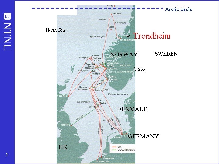
Arctic circle North Sea Trondheim NORWAY SWEDEN Oslo DENMARK GERMANY UK 5

NTNU, Trondheim 6

Outline • Control structure design (plantwide control) • A procedure for control structure design I Top Down • • Step 1: Degrees of freedom Step 2: Operational objectives (optimal operation) Step 3: What to control ? (primary CV’s) (self-optimizing control) Step 4: Where set production rate? II Bottom Up • Step 5: Regulatory control: What more to control (secondary CV’s) ? • Step 6: Supervisory control • Step 7: Real-time optimization • Case studies 7

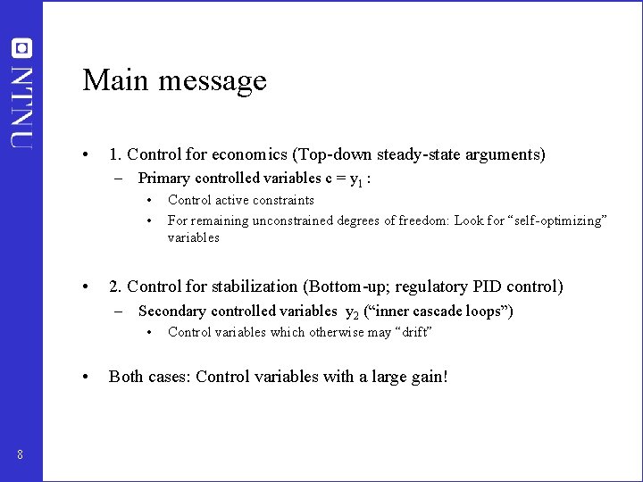
Main message • 1. Control for economics (Top-down steady-state arguments) – Primary controlled variables c = y 1 : • • • Control active constraints For remaining unconstrained degrees of freedom: Look for “self-optimizing” variables 2. Control for stabilization (Bottom-up; regulatory PID control) – Secondary controlled variables y 2 (“inner cascade loops”) • • 8 Control variables which otherwise may “drift” Both cases: Control variables with a large gain!

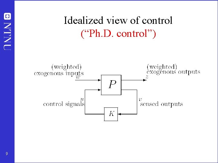
Idealized view of control (“Ph. D. control”) 9

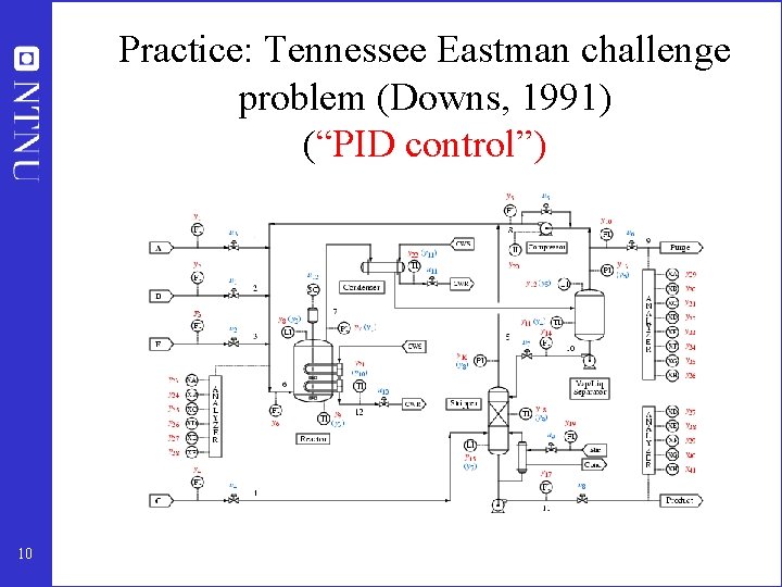
Practice: Tennessee Eastman challenge problem (Downs, 1991) (“PID control”) 10

How we design a control system for a complete chemical plant? • • 11 Where do we start? What should we control? and why? etc.

• Alan Foss (“Critique of chemical process control theory”, AICh. E Journal, 1973): The central issue to be resolved. . . is the determination of control system structure. Which variables should be measured, which inputs should be manipulated and which links should be made between the two sets? There is more than a suspicion that the work of a genius is needed here, for without it the control configuration problem will likely remain in a primitive, hazily stated and wholly unmanageable form. The gap is present indeed, but contrary to the views of many, it is theoretician who must close it. • Carl Nett (1989): Minimize control system complexity subject to the achievement of accuracy specifications in the face of uncertainty. 12

Control structure design • Not the tuning and behavior of each control loop, • But rather the control philosophy of the overall plant with emphasis on the structural decisions: – – Selection of controlled variables (“outputs”) Selection of manipulated variables (“inputs”) Selection of (extra) measurements Selection of control configuration (structure of overall controller that interconnects the controlled, manipulated and measured variables) – Selection of controller type (LQG, H-infinity, PID, decoupler, MPC etc. ). • That is: Control structure design includes all the decisions we need make to get from ``PID control’’ to “Ph. D” control 13

Process control: “Plantwide control” = “Control structure design for complete chemical plant” • • Large systems Each plant usually different – modeling expensive Slow processes – no problem with computation time Structural issues important – What to control? – Extra measurements – Pairing of loops 14

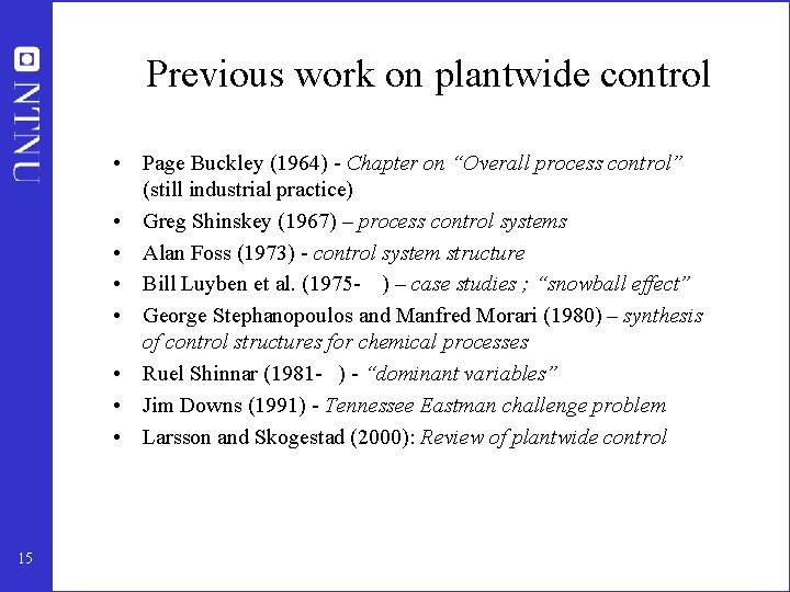
Previous work on plantwide control • Page Buckley (1964) - Chapter on “Overall process control” (still industrial practice) • Greg Shinskey (1967) – process control systems • Alan Foss (1973) - control system structure • Bill Luyben et al. (1975 - ) – case studies ; “snowball effect” • George Stephanopoulos and Manfred Morari (1980) – synthesis of control structures for chemical processes • Ruel Shinnar (1981 - ) - “dominant variables” • Jim Downs (1991) - Tennessee Eastman challenge problem • Larsson and Skogestad (2000): Review of plantwide control 15

• Control structure selection issues are identified as important also in other industries. Professor Gary Balas (Minnesota) at ECC’ 03 about flight control at Boeing: The most important control issue has always been to select the right controlled variables --- no systematic tools used! 16

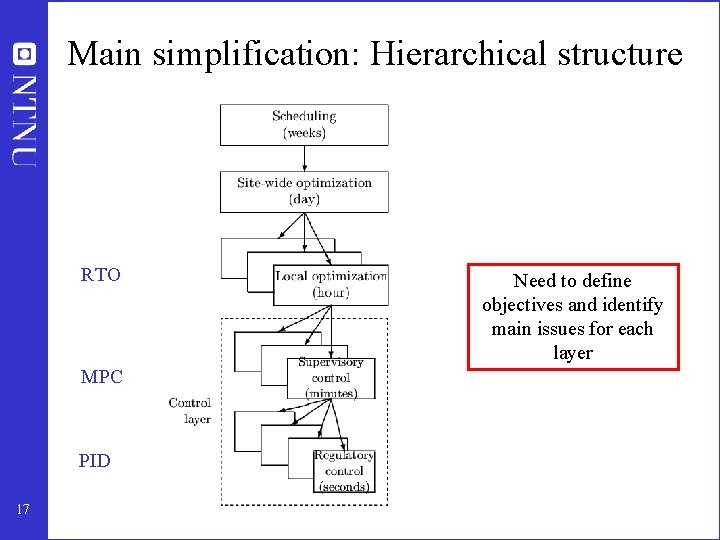
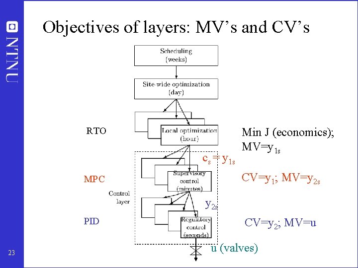
Main simplification: Hierarchical structure RTO MPC PID 17 Need to define objectives and identify main issues for each layer

Regulatory control (seconds) • Purpose: “Stabilize” the plant by controlling selected ‘’secondary’’ variables (y 2) such that the plant does not drift too far away from its desired operation • Use simple single-loop PI(D) controllers • Status: Many loops poorly tuned – Most common setting: Kc=1, I=1 min (default) – Even wrong sign of gain Kc …. 18

Regulatory control……. . . • Trend: Can do better! Carefully go through plant and retune important loops using standardized tuning procedure • Exists many tuning rules, including Skogestad (SIMC) rules: – Kc = (1/k) ( 1/ [ c + ]) I = min ( 1, 4[ c + ]), Typical: c= – “Probably the best simple PID tuning rules in the world” © Carlsberg • Outstanding structural issue: What loops to close, that is, which variables (y 2) to control? 19

Supervisory control (minutes) • Purpose: Keep primary controlled variables (c=y 1) at desired values, using as degrees of freedom the setpoints y 2 s for the regulatory layer. • Status: Many different “advanced” controllers, including feedforward, decouplers, overrides, cascades, selectors, Smith Predictors, etc. • Issues: – Which variables to control may change due to change of “active constraints” – Interactions and “pairing” 20

Supervisory control…. . . • Trend: Model predictive control (MPC) used as unifying tool. – Linear multivariable models with input constraints – Tuning (modelling) is time-consuming and expensive • Issue: When use MPC and when use simpler single-loop decentralized controllers ? – MPC is preferred if active constraints (“bottleneck”) change. – Avoids logic for reconfiguration of loops • Outstanding structural issue: – What primary variables c=y 1 to control? 21

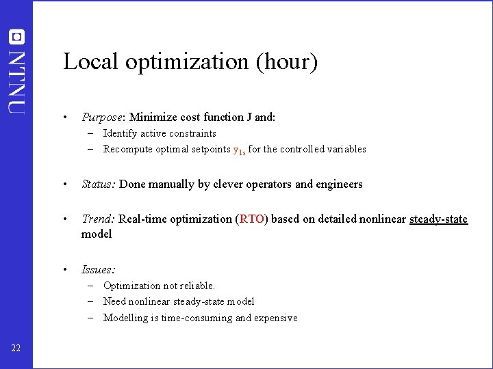
Local optimization (hour) • Purpose: Minimize cost function J and: – Identify active constraints – Recompute optimal setpoints y 1 s for the controlled variables • Status: Done manually by clever operators and engineers • Trend: Real-time optimization (RTO) based on detailed nonlinear steady-state model • Issues: – Optimization not reliable. – Need nonlinear steady-state model – Modelling is time-consuming and expensive 22

Objectives of layers: MV’s and CV’s RTO cs = y 1 s Min J (economics); MV=y 1 s CV=y 1; MV=y 2 s MPC y 2 s PID 23 CV=y 2; MV=u u (valves)

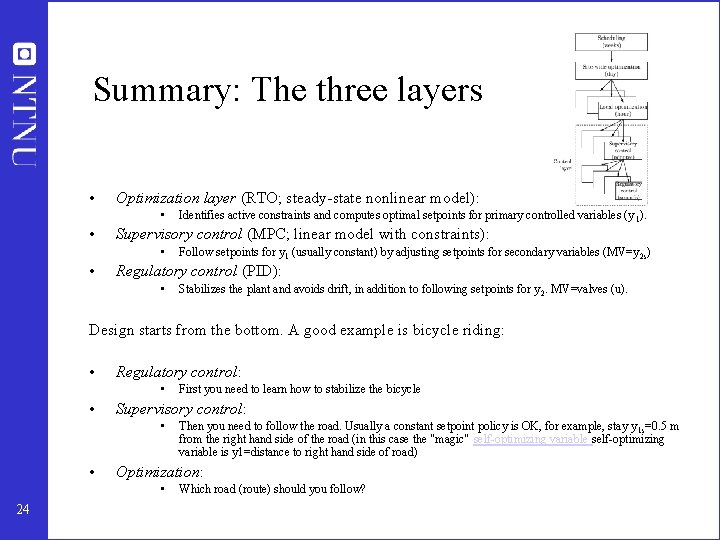
Summary: The three layers • Optimization layer (RTO; steady-state nonlinear model): • • Supervisory control (MPC; linear model with constraints): • • Identifies active constraints and computes optimal setpoints for primary controlled variables (y 1). Follow setpoints for y 1 (usually constant) by adjusting setpoints for secondary variables (MV=y 2 s) Regulatory control (PID): • Stabilizes the plant and avoids drift, in addition to following setpoints for y 2. MV=valves (u). Design starts from the bottom. A good example is bicycle riding: • Regulatory control: • • Supervisory control: • • Then you need to follow the road. Usually a constant setpoint policy is OK, for example, stay y 1 s=0. 5 m from the right hand side of the road (in this case the "magic" self-optimizing variable is y 1=distance to right hand side of road) Optimization: • 24 First you need to learn how to stabilize the bicycle Which road (route) should you follow?

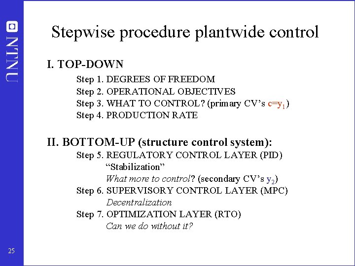
Stepwise procedure plantwide control I. TOP-DOWN Step 1. DEGREES OF FREEDOM Step 2. OPERATIONAL OBJECTIVES Step 3. WHAT TO CONTROL? (primary CV’s c=y 1) Step 4. PRODUCTION RATE II. BOTTOM-UP (structure control system): Step 5. REGULATORY CONTROL LAYER (PID) “Stabilization” What more to control? (secondary CV’s y 2) Step 6. SUPERVISORY CONTROL LAYER (MPC) Decentralization Step 7. OPTIMIZATION LAYER (RTO) Can we do without it? 25

Outline • About Trondheim and myself • Control structure design (plantwide control) • A procedure for control structure design I Top Down • • Step 1: Degrees of freedom Step 2: Operational objectives (optimal operation) Step 3: What to control ? (self-optimzing control) Step 4: Where set production rate? II Bottom Up • Step 5: Regulatory control: What more to control ? • Step 6: Supervisory control • Step 7: Real-time optimization • Case studies 26

Step 1. Degrees of freedom (DOFs) for operation (Nvalves): To find all operational (dynamic) degrees of freedom 27 • Count valves! (Nvalves) • “Valves” also includes adjustable compressor power, etc. Anything we can manipulate!

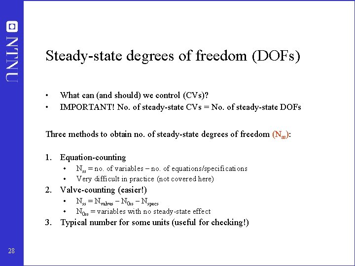
Steady-state degrees of freedom (DOFs) • • What can (and should) we control (CVs)? IMPORTANT! No. of steady-state CVs = No. of steady-state DOFs Three methods to obtain no. of steady-state degrees of freedom (Nss): 1. Equation-counting • • Nss = no. of variables – no. of equations/specifications Very difficult in practice (not covered here) 2. Valve-counting (easier!) • • Nss = Nvalves – N 0 ss – Nspecs N 0 ss = variables with no steady-state effect 3. Typical number for some units (useful for checking!) 28

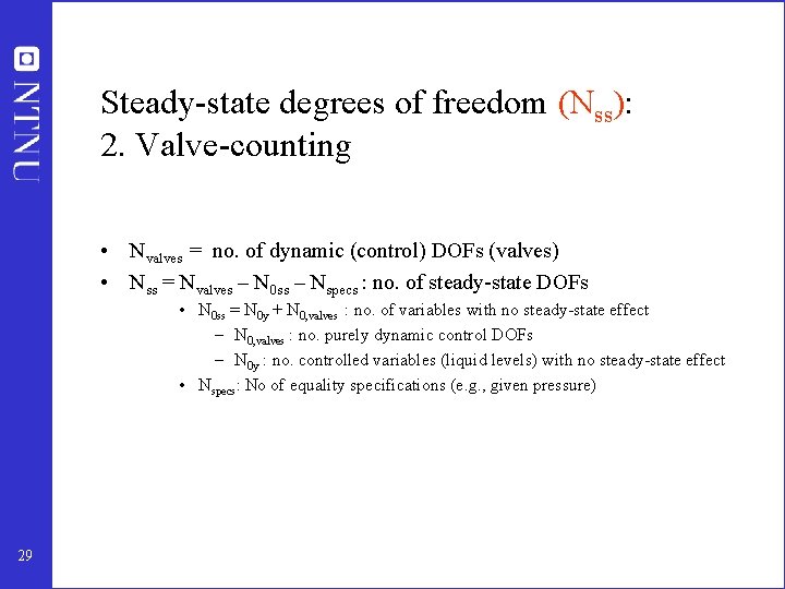
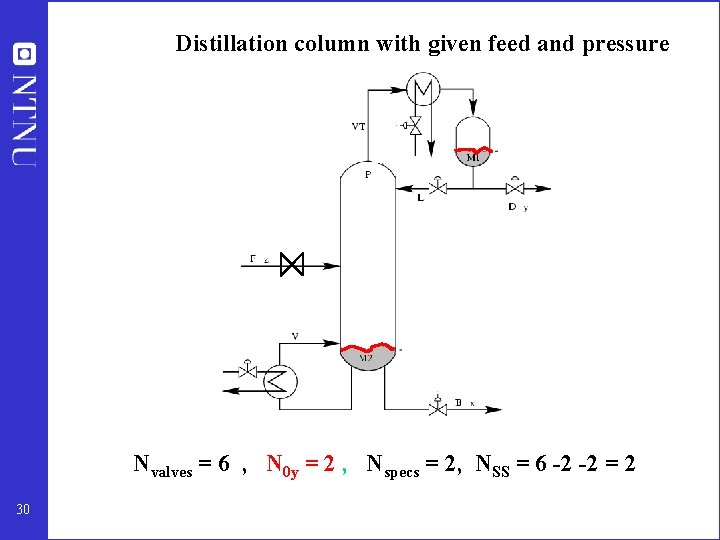
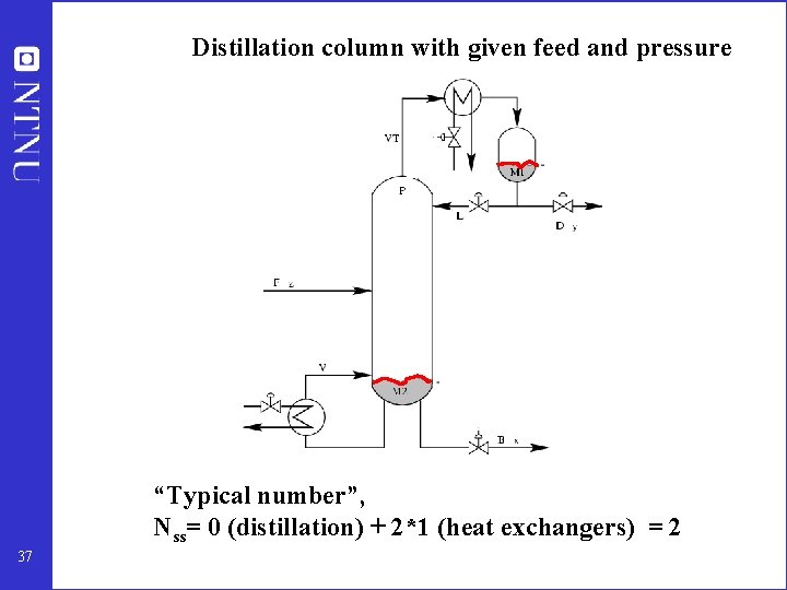
Steady-state degrees of freedom (Nss): 2. Valve-counting • Nvalves = no. of dynamic (control) DOFs (valves) • Nss = Nvalves – N 0 ss – Nspecs : no. of steady-state DOFs • N 0 ss = N 0 y + N 0, valves : no. of variables with no steady-state effect – N 0, valves : no. purely dynamic control DOFs – N 0 y : no. controlled variables (liquid levels) with no steady-state effect • Nspecs: No of equality specifications (e. g. , given pressure) 29

Distillation column with given feed and pressure Nvalves = 6 , N 0 y = 2 , Nspecs = 2, NSS = 6 -2 -2 = 2 30

Heat-integrated distillation process 31

Heat-integrated distillation process 32

Heat exchanger with bypasses 33

Heat exchanger with bypasses 34

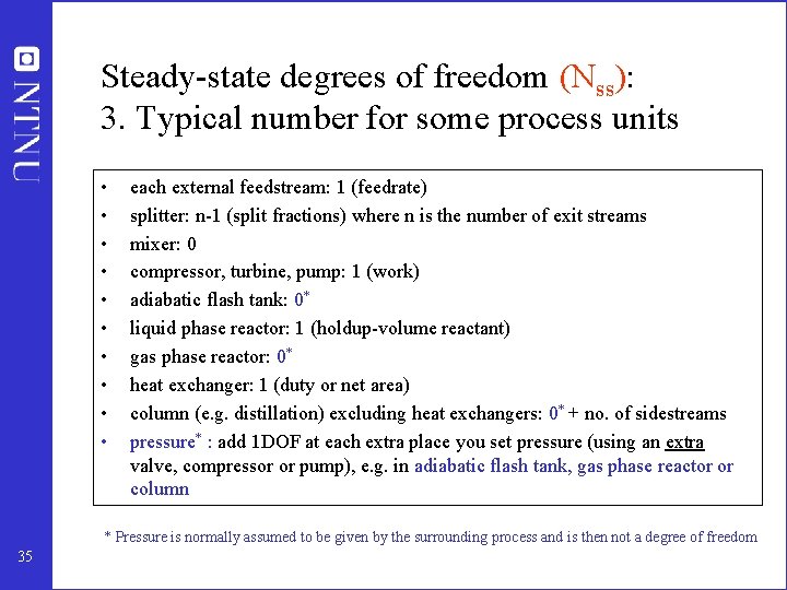
Steady-state degrees of freedom (Nss): 3. Typical number for some process units • • • each external feedstream: 1 (feedrate) splitter: n-1 (split fractions) where n is the number of exit streams mixer: 0 compressor, turbine, pump: 1 (work) adiabatic flash tank: 0* liquid phase reactor: 1 (holdup-volume reactant) gas phase reactor: 0* heat exchanger: 1 (duty or net area) column (e. g. distillation) excluding heat exchangers: 0* + no. of sidestreams pressure* : add 1 DOF at each extra place you set pressure (using an extra valve, compressor or pump), e. g. in adiabatic flash tank, gas phase reactor or column * Pressure is normally assumed to be given by the surrounding process and is then not a degree of freedom 35

Heat exchanger with bypasses 36

Distillation column with given feed and pressure “Typical number”, Nss= 0 (distillation) + 2*1 (heat exchangers) = 2 37

Heat-integrated distillation process 38

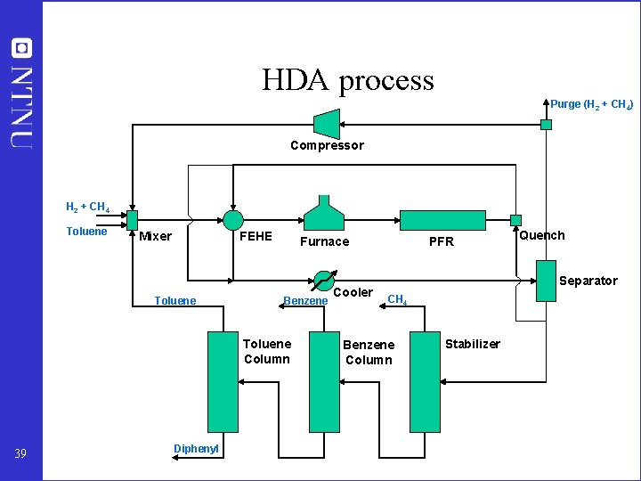
HDA process Purge (H 2 + CH 4) Compressor H 2 + CH 4 Toluene Mixer FEHE Toluene Furnace Benzene Toluene Column 39 Diphenyl Cooler PFR Quench Separator CH 4 Benzene Column Stabilizer

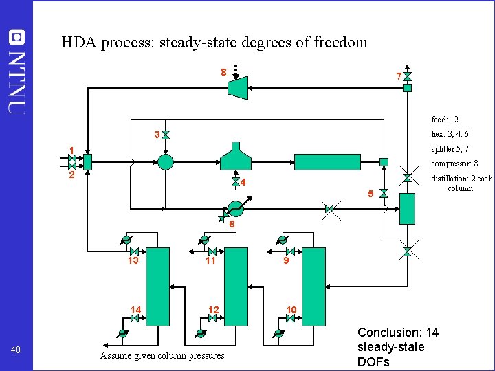
HDA process: steady-state degrees of freedom 8 7 feed: 1. 2 3 hex: 3, 4, 6 splitter 5, 7 1 compressor: 8 2 4 5 distillation: 2 each column 6 40 13 11 9 14 12 10 Assume given column pressures Conclusion: 14 steady-state DOFs

• Check that there are enough manipulated variables (DOFs) - both dynamically and at steady-state (step 2) • Otherwise: Need to add equipment – extra heat exchanger – bypass – surge tank 41