Physics 736 Experimental Methods in Nuclear Particle and

Physics 736: Experimental Methods in Nuclear, Particle, and Astro Physics Prof. Vandenbroucke, April 27, 2015

Announcements • Written document for report (extended outline with figures and references) due Thu (Apr 30): email to me by 5 pm • Office hours Wed 3: 45 -4: 45 (Chamberlin 4114) • Read Barlow 8. 5 -10. 4 for Wed (Apr 29) • Presentations start one week from today • Online course evaluations are available April 29 until May 13: please do these (and put some thought into them)!

Fitting a histogram with empty bins • Three methods (see Bevington & Robinson) 1. Use standard chi-squared with errors equal to sqrt of measured counts, ignoring empty bins (their error would give division by zero). Advantage: analytical solution. Disadvantage: we ignore the information that the empty bins is telling us, introducing bias. Good when most bins have at least 10 counts and there are few empty bins. 2. Use chi-squared, but with errors equal to sqrt of model counts. Advantage: includes information from empty bins. Disadvantage: model is now in both numerator and denominator, so typically no analytical solution. Probably better to use (1) or (3) 3. Use likelihood fit based on Poisson rather than Gaussian distribution for each data point, with errors equal to sqrt of model counts. Advantage: fully general solution, correct for large, small, and zero counts. Disadvantage: no analytical solution. Good to use when empty bins provide important constraint and/or many bins have small count

Conditional probability Define two events A and B P(A) is the probability of A occurring P(B) is the probability of B occurring P(A|B) is the probability of A occurring given that B occurs • P(B and A) = P(B)*P(A|B) • Can be viewed in terms of set theory and Venn diagrams • •

Example: cards • A card is drawn from a fair deck of 52. What is the probability it is a spade? P(A) = 13/52 = 1/4 • A second card is drawn from the deck. What is the probability it is a spade? – If we do not know what the first card was, it is P(B) = 13/52 = 1/4 – If we know the first card was a spade, it is 12/51 • What is the probability that the first two cards are both spades? – P(A and B) = P(A) * P(B|A) = (1/4)*(12/51) = 5. 9% • Note that the probability we assign to an event depends not only on the event itself but on any other information we have that may be relevant: external/prior knowledge modifies our degree of belief that the event will occur

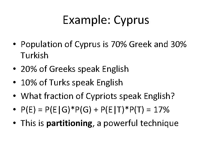
Example: Cyprus • Population of Cyprus is 70% Greek and 30% Turkish • 20% of Greeks speak English • 10% of Turks speak English • What fraction of Cypriots speak English? • P(E) = P(E|G)*P(G) + P(E|T)*P(T) = 17% • This is partitioning, a powerful technique

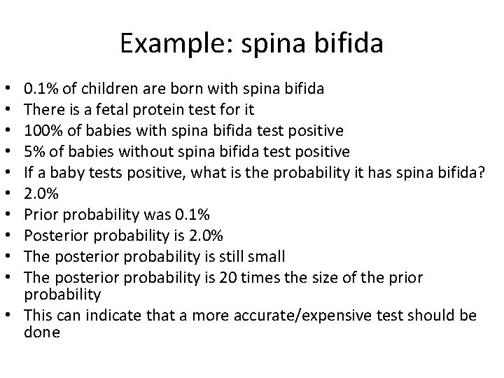
Example: spina bifida 0. 1% of children are born with spina bifida There is a fetal protein test for it 100% of babies with spina bifida test positive 5% of babies without spina bifida test positive If a baby tests positive, what is the probability it has spina bifida? 2. 0% Prior probability was 0. 1% Posterior probability is 2. 0% The posterior probability is still small The posterior probability is 20 times the size of the prior probability • This can indicate that a more accurate/expensive test should be done • • •

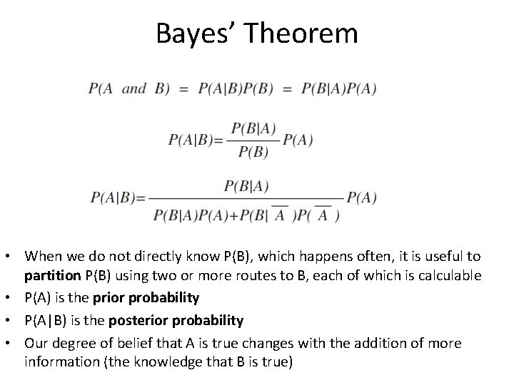
Bayes’ Theorem • When we do not directly know P(B), which happens often, it is useful to partition P(B) using two or more routes to B, each of which is calculable • P(A) is the prior probability • P(A|B) is the posterior probability • Our degree of belief that A is true changes with the addition of more information (the knowledge that B is true)

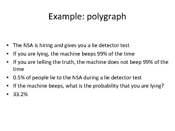
Example: polygraph • The NSA is hiring and gives you a lie detector test • If you are lying, the machine beeps 99% of the time • If you are telling the truth, the machine does not beep 99% of the time • 0. 5% of people lie to the NSA during a lie detector test • If the machine beeps, what is the probability that you are lying? • 33. 2%

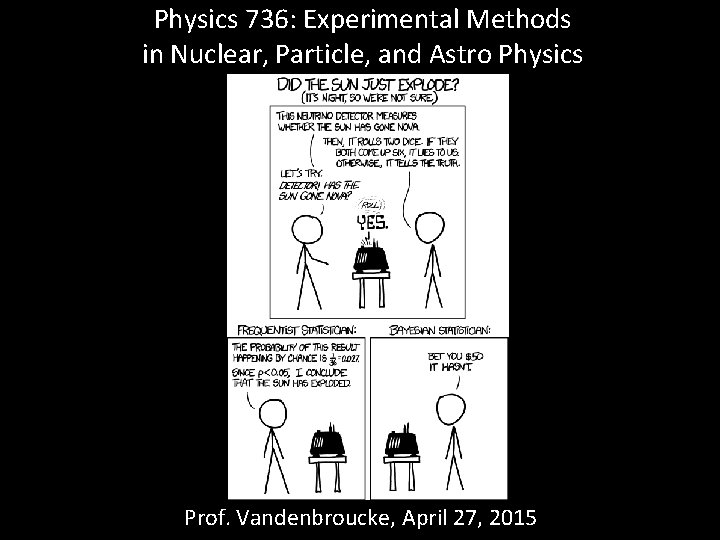
Bayesian statistics • Bayes’ Theorem can be used fully within frequentist statistics when A and B are both events • When A or B is a hypothesis rather than an event, the two schools of thought diverge • In Bayesian/subjective statistics (specifically, Bayesian inference), we can assign a probability to a hypothesis and interpret it as degree of belief that the hypothesis is true • Bayesian inference: quantitative method for updating our degree of belief in a hypothesis as more information is acquired

Bayesian inference example (from Nate Silver, The Signal and the Noise) • You return from a business trip and discover a strange pair of underwear in your boyfriend’s drawer. What is the probability that he is cheating on you? • Definitions – C: he is cheating – F: he is faithful (not cheating) – U: you found the underwear • P(U|C) = 0. 5 • P(U|F) = 0. 05 • P(C) = 0. 04 • Using Bayes’ Theorem, P(C|U) = 29%

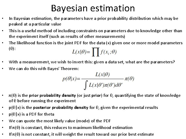
Bayesian estimation • • • In Bayesian estimation, the parameters have a prior probability distribution which may be peaked at a particular value This is a useful method of including constraints on parameters due to knowledge other than the experiment itself (such as results of other measurements) The likelihood function is the joint PDF for the data (x) given one or more model parameters (θ): • • With a measurement, we wish to invert this: given a data set, what are the parameters? We can do this with Bayes’ Theorem: • π(θ) is the prior probability density (or just prior) for θ, quantifying the state of knowledge of θ before running the experiment p(θ|x) is the posterior probability density for θ, given the experimental results p(θ|x) is a PDF for theta We can quote the most likely value (mode) of the PDF If π(θ) is constant, this reduces to maximum likelihood estimation If π(θ) is not constant, it will weight the result toward our prior best estimate • • •

Notes on Bayesian estimation • A prior PDF that is uniform in a particular parameter is not necessarily uniform under a transformation of that parameter! • So it is difficult to choose a prior that universally expresses ignorance, e. g. choosing a uniform prior for θ means that the prior for θ 2 is not uniform, and there is no clear reason that either one is the “natural” parameter for the problem • Maximum likelihood estimation is invariant under parameter transformation, but Bayesian estimation is not

Hypothesis testing • We’ve worked a lot on parameter estimation: given a data set and a model, find the best estimate for the parameters of the model • Another class of questions (sometimes even more important) is to answer a yes or no question – Do the data fit the model? – Is there signal present (or only background)? – Are these two samples from the same distribution? – Does this medicine perform better than a placebo? • Procedure: state a hypothesis clearly and as simply as possible, then devise a test that will accept or reject the hypothesis based on the data • You will not always answer the question correctly • You can quantify the probability of answering incorrectly (in both possible ways) • You can design the test to choose a tradeoff between these possible incorrect answers

Hypothesis testing: 4 possible outcomes • A hypothesis is true, and you accept it (correctly) • A hypothesis is false, and you reject it (correctly) • A hypothesis is true, and you reject it (incorrectly) – False negative, aka Type I error • A hypothesis is false, and you accept it (incorrectly) – False positive, aka Type II error

Hypothesis testing for determining whethere is signal present in background/noise • It is generally not possible to prove that a signal does not exist, only that it is small (e. g. , below some value at some confidence level) • Define a null hypothesis: “The measured data are consistent with background” • The alternative hypothesis is then “The measured data are inconsistent with background” • In a simple/idealized experiment, the alternative hypothesis is identical to the hypothesis “signal is present” but in reality there are often multiple alternative hypotheses • To discover a signal, we need to reject the null hypothesis (at some confidence level) • What is the probability of falsely rejecting the null hypothesis (false discovery? ) • What is the probability of falsely accepting the null hypothesis (missing a discovery? )

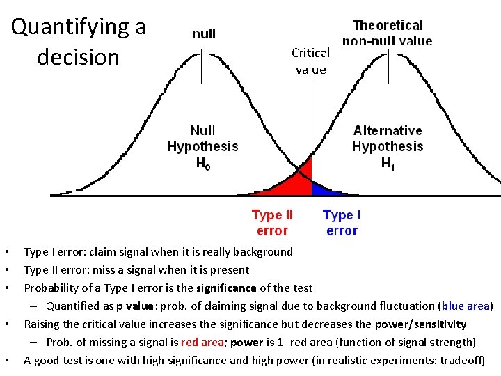
Quantifying a decision • • • Critical value Type I error: claim signal when it is really background Type II error: miss a signal when it is present Probability of a Type I error is the significance of the test – Quantified as p value: prob. of claiming signal due to background fluctuation (blue area) Raising the critical value increases the significance but decreases the power/sensitivity – Prob. of missing a signal is red area; power is 1 - red area (function of signal strength) A good test is one with high significance and high power (in realistic experiments: tradeoff)