Physics 736 Experimental Methods in Nuclear Particle and

Physics 736: Experimental Methods in Nuclear, Particle, and Astro Physics Prof. Vandenbroucke, April 6, 2015

Physics 736: Experimental Methods in Nuclear, Particle, and Astro Physics Prof. Vandenbroucke, April 6, 2015

Physics 736: Experimental Methods in Nuclear, Particle, and Astro Physics Prof. Vandenbroucke, April 6, 2015

Announcements • Project proposals due today at 5 pm – See details in project handout (posted on learn@uw) – Send me email – 1 -2 paragraphs is fine – If working in group, name group members • Start working on projects! • Problem Set 8 due Thursday 5 pm • No problem set next week: work on projects • Office hours today (not Wed) 3: 45 -4: 45 (Chamberlin 4114) • Read Barlow 4. 3 -5. 1 for Wed (Apr 8) • Read Barlow 5. 2 -5. 3 for Mon (Apr 13)

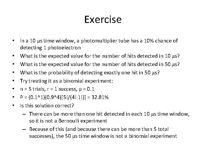
Exercise • In a 10 µs time window, a photomultiplier tube has a 10% chance of detecting 1 photoelectron • What is the expected value for the number of hits detected in 10 µs? • What is the expected value for the number of hits detected in 50 µs? • What is the probability of detecting exactly one hit in 50 µs? • Try treating it as a binomial experiment: • n = 5 trials, r = 1 success, p = 0. 1 • P = (0. 1^1)(0. 9^4)[5!/(4! 1!)] = 32. 81% • Is this solution correct? – There can be more than one hit detected in each 10 µs time window, so it is not a Bernoulli experiment – Because of this (and because there can be more than 5 total successes), the 50 µs time window is not a binomial experiment

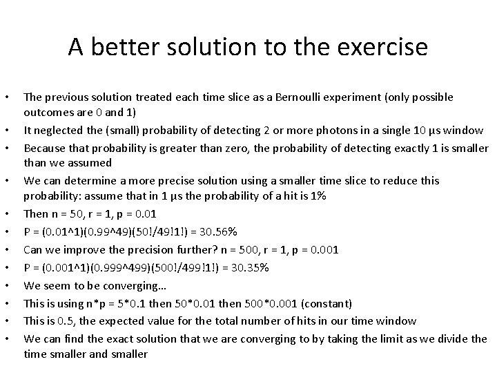
A better solution to the exercise • • • The previous solution treated each time slice as a Bernoulli experiment (only possible outcomes are 0 and 1) It neglected the (small) probability of detecting 2 or more photons in a single 10 µs window Because that probability is greater than zero, the probability of detecting exactly 1 is smaller than we assumed We can determine a more precise solution using a smaller time slice to reduce this probability: assume that in 1 µs the probability of a hit is 1% Then n = 50, r = 1, p = 0. 01 P = (0. 01^1)(0. 99^49)(50!/49!1!) = 30. 56% Can we improve the precision further? n = 500, r = 1, p = 0. 001 P = (0. 001^1)(0. 999^499)(500!/499!1!) = 30. 35% We seem to be converging… This is using n*p = 5*0. 1 then 50*0. 01 then 500*0. 001 (constant) This is 0. 5, the expected value for the total number of hits in our time window We can find the exact solution that we are converging to by taking the limit as we divide the time smaller and smaller

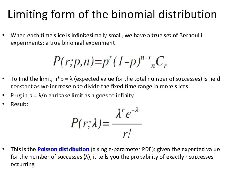
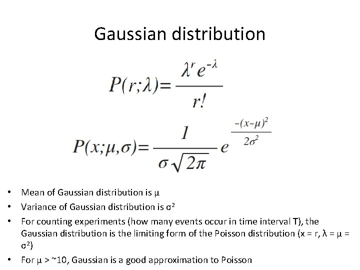
Limiting form of the binomial distribution • When each time slice is infinitesimally small, we have a true set of Bernoulli experiments: a true binomial experiment • To find the limit, n*p = λ (expected value for the total number of successes) is held constant as we increase n to divide the fixed time range in more slices • Plug in p = λ/n and take limit as n goes to infinity • Result: • This is the Poisson distribution (a single-parameter PDF): given the expected value for the number of successes (λ), it tells you the probability of exactly r successes occurring

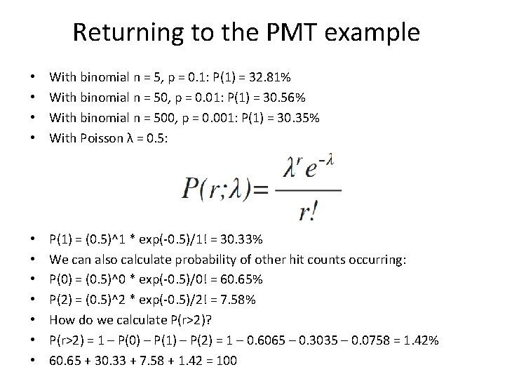
Returning to the PMT example • • With binomial n = 5, p = 0. 1: P(1) = 32. 81% With binomial n = 50, p = 0. 01: P(1) = 30. 56% With binomial n = 500, p = 0. 001: P(1) = 30. 35% With Poisson λ = 0. 5: • • P(1) = (0. 5)^1 * exp(-0. 5)/1! = 30. 33% We can also calculate probability of other hit counts occurring: P(0) = (0. 5)^0 * exp(-0. 5)/0! = 60. 65% P(2) = (0. 5)^2 * exp(-0. 5)/2! = 7. 58% How do we calculate P(r>2)? P(r>2) = 1 – P(0) – P(1) – P(2) = 1 – 0. 6065 – 0. 3035 – 0. 0758 = 1. 42% 60. 65 + 30. 33 + 7. 58 + 1. 42 = 100

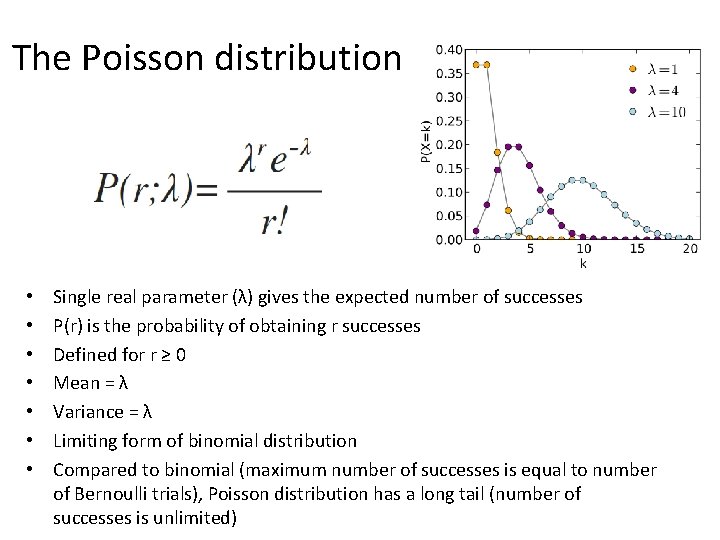
The Poisson distribution • • Single real parameter (λ) gives the expected number of successes P(r) is the probability of obtaining r successes Defined for r ≥ 0 Mean = λ Variance = λ Limiting form of binomial distribution Compared to binomial (maximum number of successes is equal to number of Bernoulli trials), Poisson distribution has a long tail (number of successes is unlimited)

Poisson process • Any random process characterized by events occurring with constant probability of occurrence per unit time • Number of events in any time interval (large or small) is described by Poisson distribution • For the probability of occurrence per unit time to be independent of the time interval, events must be independent of one another • Many processes in particle, nuclear, astro are Poisson processes • Correlated events are not Poisson (e. g. the positron and neutron events from inverse beta decay) • Poisson processes have no “memory”: probability per unit time remains constant regardless of past behavior (such as time since last event) • Given rate r, probability of occurrence of an event in differential time interval dt is dp = r dt • For finite time interval T, average number of events occurring is r T • Example Poisson processes: radioactive decays, photon detections in a photosensor, Higgs production events (on time scales much larger than bunch crossing time), telephone calls arriving at cell tower

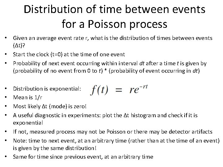
Distribution of time between events for a Poisson process • Given an average event rate r, what is the distribution of times between events (Δt)? • Start the clock (t=0) at the time of one event • Probability of next event occurring within interval dt after a time t is given by (probability of no event from 0 to t) * (probability of event occurring in dt) Distribution is exponential: Mean is 1/r Most likely Δt (mode) is zero! A useful diagnostic in experiments: plot the Δt histogram and check if it is exponential • If not, measured process may not be Poisson or there may be detector artifacts • Note: time to next event, at an arbitrary time (rather than at the time of an event) is given by the same distribution! • Same for time since previous event, at an arbitrary time • •

Gaussian distribution • Mean of Gaussian distribution is µ • Variance of Gaussian distribution is σ2 • For counting experiments (how many events occur in time interval T), the Gaussian distribution is the limiting form of the Poisson distribution (x = r, λ = µ = σ2 ) • For µ > ~10, Gaussian is a good approximation to Poisson

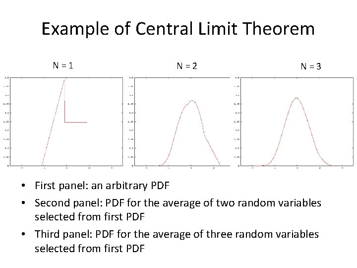
Central limit theorem • Given N independent random variables xi, each with any arbitrary distribution function, not necessarily all the same function • Each random variable has mean µi and variance Vi • Let X (another random variable) be the sum of xi • Central Limit Theorem: 1. Expectation value of X is sum of µi 2. Variance of X is sum of Vi (Bienaymé Formula) 3. X is Gaussian distributed in the limit of large N (even though xi are arbitrarily distributed) • This is why Gaussian distributions are so ubiquitous: arises any time many independent effects sum together, no matter what the shape of the independent effects • This is why measurement errors are often Gaussian: several independent effects sum together

Example of Central Limit Theorem N=1 N=2 N=3 • First panel: an arbitrary PDF • Second panel: PDF for the average of two random variables selected from first PDF • Third panel: PDF for the average of three random variables selected from first PDF

Combining measurements with the same uncertainty • If a measurement is repeated N times with each measurement having the same uncertainty σ, then • The best estimate is given by the mean of the individual estimates • Because the variances sum, the uncertainty on the overall best estimate is given by σ/sqrt(N)

Combining measurements each with a different uncertainty • If each measurement is xi ± σi, then the best estimate obtained by combining results is given by weighting them according to the uncertainty squared: • wi = 1/σi 2 • The best estimate is x = sum(xiwi)/sum(wi) • Uncertainty of best estimate is given by σ2 = 1/sum(wi)