Physics 736 Experimental Methods in Nuclear Particle and

Physics 736: Experimental Methods in Nuclear, Particle, and Astro Physics Prof. Vandenbroucke, April 15, 2015

Announcements • No problem set this week: work on projects • Written document for report (extended outline + figures) due Thu Apr 30 • Office hours today 3: 45 -4: 45 (Chamberlin 4114) • Read Barlow 6. 5 -7. 1 for Mon (Apr 20) • Read Barlow 7. 2 -8. 1 for Wed (Apr 22)

Final presentation schedule • May 4 – Kevin M – Richard – Kevin G – Andrew • May 6 – Robert – Erin – Sam – Zach • May 13 – Sida – Jiande – Kenneth – Nick – Matt – Tyler – Shaun • Each presentation will be 13 min + 3 min for questions • For group projects, each person should give a presentation

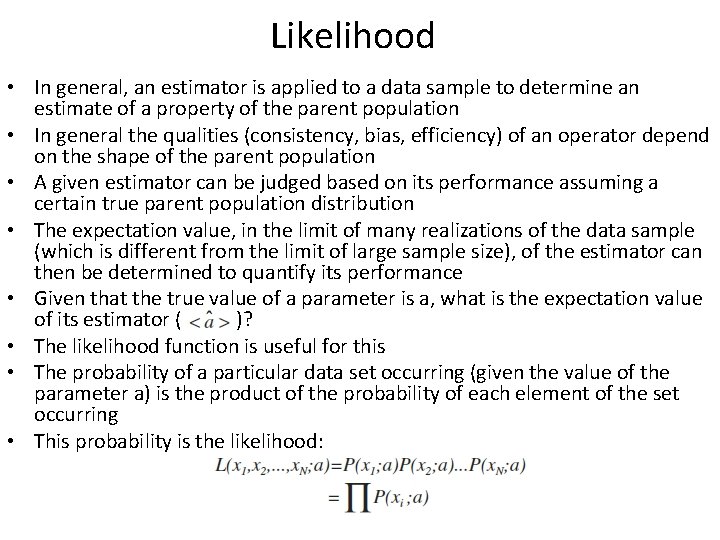
Likelihood • In general, an estimator is applied to a data sample to determine an estimate of a property of the parent population • In general the qualities (consistency, bias, efficiency) of an operator depend on the shape of the parent population • A given estimator can be judged based on its performance assuming a certain true parent population distribution • The expectation value, in the limit of many realizations of the data sample (which is different from the limit of large sample size), of the estimator can then be determined to quantify its performance • Given that the true value of a parameter is a, what is the expectation value of its estimator ( )? • The likelihood function is useful for this • The probability of a particular data set occurring (given the value of the parameter a) is the product of the probability of each element of the set occurring • This probability is the likelihood:

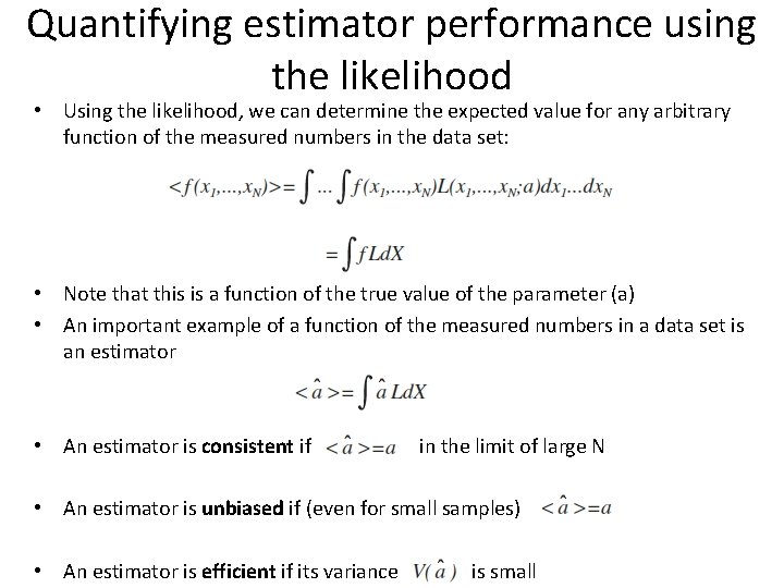
Quantifying estimator performance using the likelihood • Using the likelihood, we can determine the expected value for any arbitrary function of the measured numbers in the data set: • Note that this is a function of the true value of the parameter (a) • An important example of a function of the measured numbers in a data set is an estimator • An estimator is consistent if in the limit of large N • An estimator is unbiased if (even for small samples) • An estimator is efficient if its variance is small

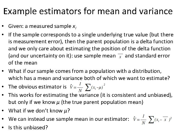
Example estimators for mean and variance • Given: a measured sample xi • If the sample corresponds to a single underlying true value (but there is measurement error), then the parent population is a delta function and we only care about estimating the position of the delta function (and our uncertainty on it): use sample mean and standard error of the mean • What if our sample comes from a population with a distribution, which has a mean and variance both of which we want to estimate? • The obvious estimator is • This works for estimating the variance (it is consistent and unbiased), but only if we know µ (the true parent population mean) • What if we don’t know µ? • We can instead use sample mean in our estimator: • Is this unbiased?

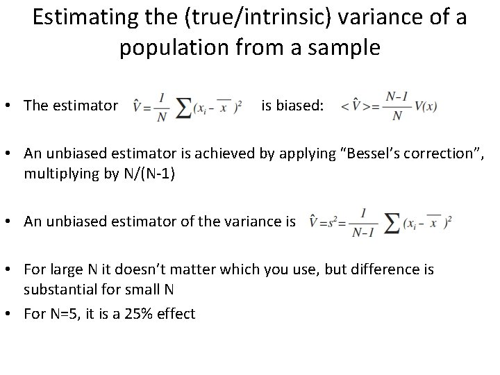
Estimating the (true/intrinsic) variance of a population from a sample • The estimator is biased: • An unbiased estimator is achieved by applying “Bessel’s correction”, multiplying by N/(N-1) • An unbiased estimator of the variance is • For large N it doesn’t matter which you use, but difference is substantial for small N • For N=5, it is a 25% effect

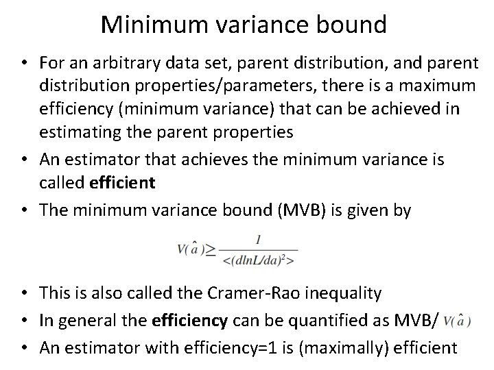
Minimum variance bound • For an arbitrary data set, parent distribution, and parent distribution properties/parameters, there is a maximum efficiency (minimum variance) that can be achieved in estimating the parent properties • An estimator that achieves the minimum variance is called efficient • The minimum variance bound (MVB) is given by • This is also called the Cramer-Rao inequality • In general the efficiency can be quantified as MVB/ • An estimator with efficiency=1 is (maximally) efficient

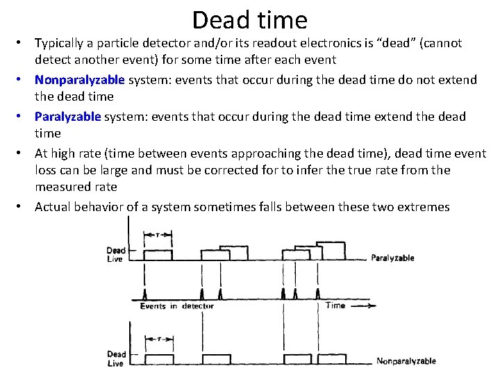
Dead time • Typically a particle detector and/or its readout electronics is “dead” (cannot detect another event) for some time after each event • Nonparalyzable system: events that occur during the dead time do not extend the dead time • Paralyzable system: events that occur during the dead time extend the dead time • At high rate (time between events approaching the dead time), dead time event loss can be large and must be corrected for to infer the true rate from the measured rate • Actual behavior of a system sometimes falls between these two extremes