Perfect Competition Udayan Roy ECO 10 Introduction to

Perfect Competition Udayan Roy ECO 10 Introduction to Microeconomics

Sources: Principles of Microeconomics/Economics by N. Gregory Mankiw • Chapter 14: Firms in Competitive Markets

Sources: Principles of Microeconomics/Economics by Timothy Taylor • Chapter 10: Perfect Competition

Sources: The Economy by The CORE Team • Unit 8: Supply and demand: Price-taking and competitive markets ELASTICITY 4

Perfect Competition • In a perfectly competitive market • There are many buyers • There are many sellers • In the long run, firms can freely enter or exit the market • In the short run, the number of firms is assumed fixed (constant). • All sellers sell the same product.

Perfect Competition • As a result: • The actions of any single buyer or seller have a negligible impact on the market price. • That is, the market price is unaffected by the amount bought by a buyer or the amount sold by a seller • Therefore, every buyer and every seller takes the market price as given. • Everybody is a ‘price taker’

Everyone is a “price taker” • A firm in a perfectly competitive market cannot stay in business if its price is higher than what the other firms are charging • No firm would be able to raise the market price by reducing production and attempting to create a shortage. • Conversely, there is no danger that a firm would drive the market price down by producing too much. • Therefore, no firm would want to charge a price lower than what the others are charging. • In short, each firm takes the prevailing market price as a given—like the weather—and charges that price.

Demand

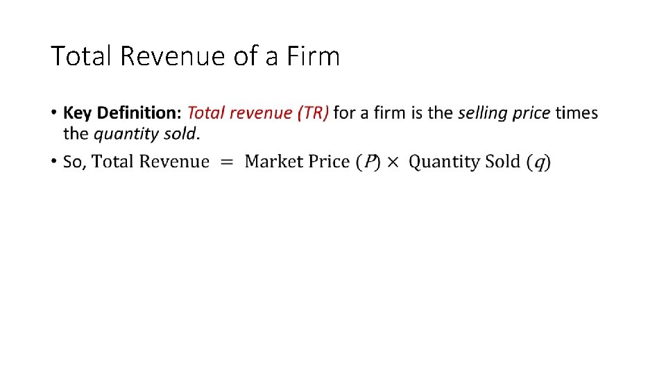
Total Revenue of a Firm •

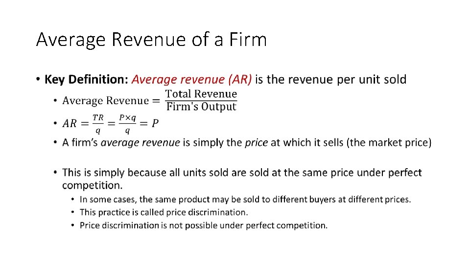
Average Revenue of a Firm •

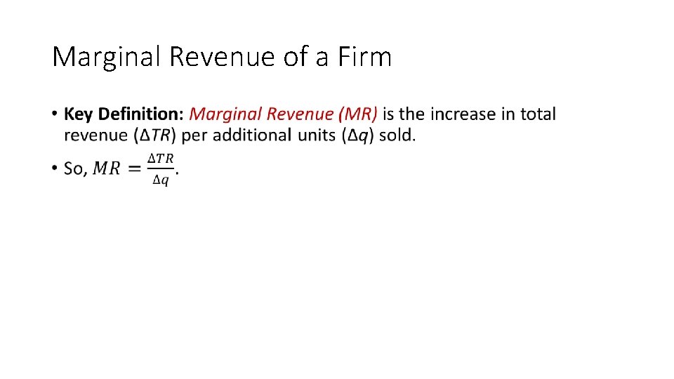
Marginal Revenue of a Firm •

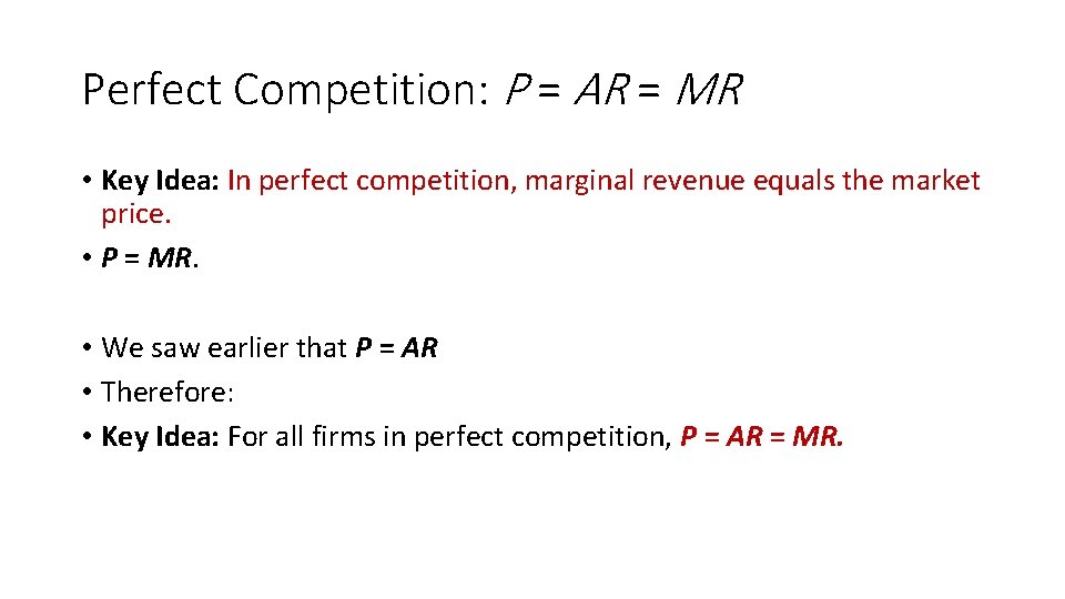
Perfect Competition: P = AR = MR • Key Idea: In perfect competition, marginal revenue equals the market price. • P = MR. • We saw earlier that P = AR • Therefore: • Key Idea: For all firms in perfect competition, P = AR = MR.

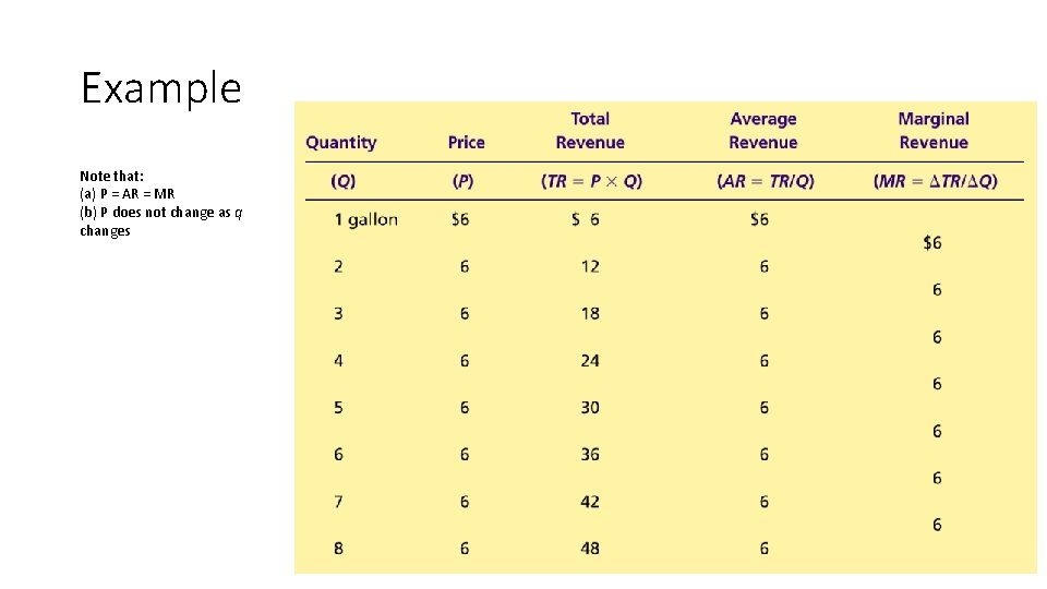
Example Note that: (a) P = AR = MR (b) P does not change as q changes

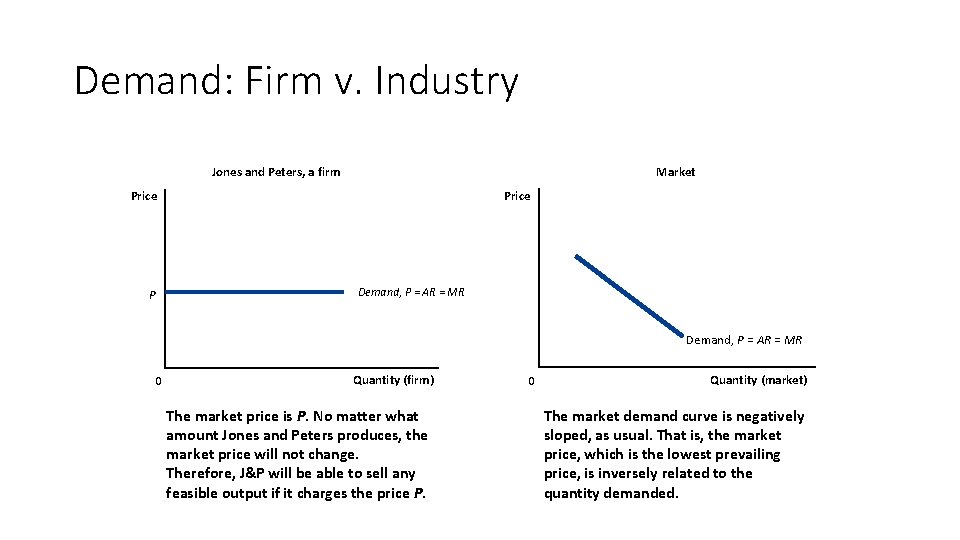
Demand: Firm v. Industry Market Jones and Peters, a firm Price Demand, P = AR = MR P Demand, P = AR = MR 0 Quantity (firm) The market price is P. No matter what amount Jones and Peters produces, the market price will not change. Therefore, J&P will be able to sell any feasible output if it charges the price P. 0 Quantity (market) The market demand curve is negatively sloped, as usual. That is, the market price, which is the lowest prevailing price, is inversely related to the quantity demanded.

Supply We have just seen the demand curves for a firm and for the entire industry Next, we need to work out what the supply curves look like

Supply: short run and long run • The analysis of supply in perfect competition depends on whether it is the short run or the long run.

Short run and long run: assumptions • Key Assumption: All fixed costs are sunk costs in the short run, but not in the long run • Definition: Sunk costs are costs that are unavoidable even when production is zero • Key Assumption: The number of firms in an industry is fixed in the short run, but not in the long run

Supply / Short Run Stay Open or Shut Down Temporarily?

Shut Down and Exit • Before a firm decides how much to produce, it must decide whether or not to stay in business • Key definition: A shutdown refers to a short-run decision to stop production temporarily, perhaps because of poor market conditions. • Key definition: An exit refers to a long-run decision to end production permanently and leave the industry.

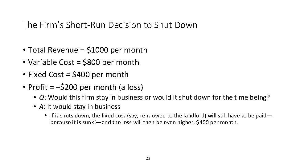
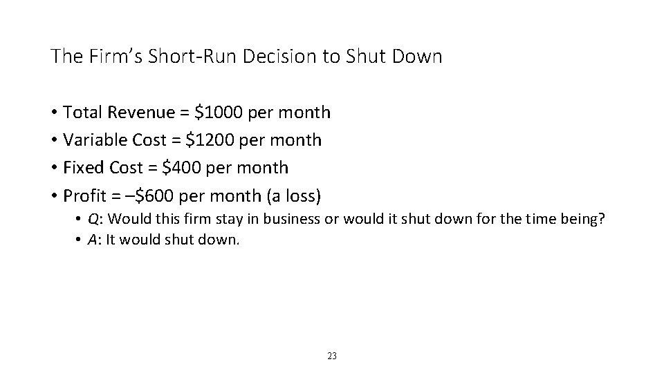
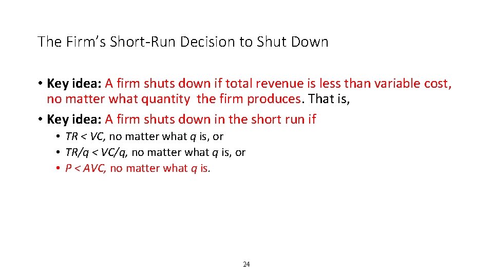
The Firm’s Short-Run Decision to Shut Down • Key idea: A firm will shut down (temporarily) if its variable costs exceed its total revenue, no matter what quantity it produces • Its fixed costs do not matter! • This is because • Fixed costs are sunk costs in the short run • sunk costs are defined as costs that will have to be paid even if the firm shuts down. • Therefore, FC cannot affect a firm’s decision on whether to stay open or shut down 20

Sunk Costs • Sunk costs will have to be paid even when a firm is in a temporary shutdown. • Examples: • If the firm signs a long-term contract with its landlord, the rent will have to be paid even when the firm is temporarily shut down. • Some maintenance costs will have to be incurred even when the firm is shut down. • The firm may be under contract to provide customer service to past customers even after it shuts down. 21

The Firm’s Short-Run Decision to Shut Down • Total Revenue = $1000 per month • Variable Cost = $800 per month • Fixed Cost = $400 per month • Profit = –$200 per month (a loss) • Q: Would this firm stay in business or would it shut down for the time being? • A: It would stay in business • If it shuts down, the fixed cost (say, rent owed to the landlord) will still have to be paid— because it is sunk!—and the loss will then be even higher, $400 per month. 22

The Firm’s Short-Run Decision to Shut Down • Total Revenue = $1000 per month • Variable Cost = $1200 per month • Fixed Cost = $400 per month • Profit = –$600 per month (a loss) • Q: Would this firm stay in business or would it shut down for the time being? • A: It would shut down. 23

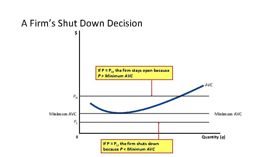
The Firm’s Short-Run Decision to Shut Down • Key idea: A firm shuts down if total revenue is less than variable cost, no matter what quantity the firm produces. That is, • Key idea: A firm shuts down in the short run if • TR < VC, no matter what q is, or • TR/q < VC/q, no matter what q is, or • P < AVC, no matter what q is. 24

A Firm’s Shut Down Decision $ If P = PH, the firm stays open because P > Minimum AVC PH Minimum AVC PL Quantity (q) 0 If P = PL, the firm shuts down because P < Minimum 25 AVC

Profit Maximization

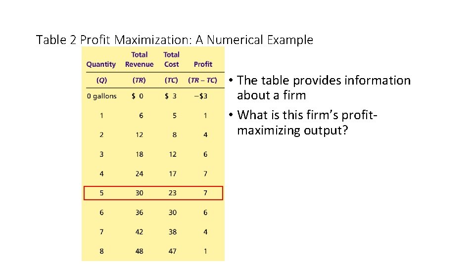
Table 2 Profit Maximization: A Numerical Example • The table provides information about a firm • What is this firm’s profitmaximizing output?

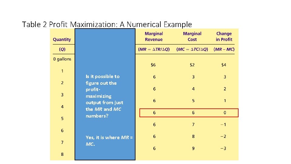
Table 2 Profit Maximization: A Numerical Example Is it possible to figure out the profitmaximizing output from just the MR and MC numbers? Yes, it is where MR = MC. 28

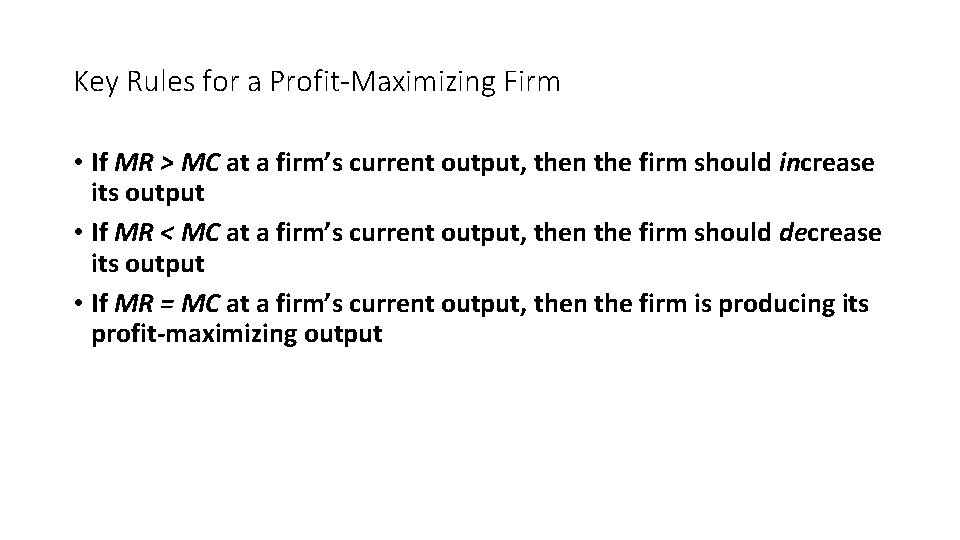
Key Rules for a Profit-Maximizing Firm • If MR > MC at a firm’s current output, then the firm should increase its output • If MR < MC at a firm’s current output, then the firm should decrease its output • If MR = MC at a firm’s current output, then the firm is producing its profit-maximizing output

Key Rules for a Profit-Maximizing Firm • Profit maximization occurs at the quantity where marginal revenue equals marginal cost. • This is a crucial principle in understanding the behavior of firms

Profit-maximization by a firm in a perfectly competitive industry

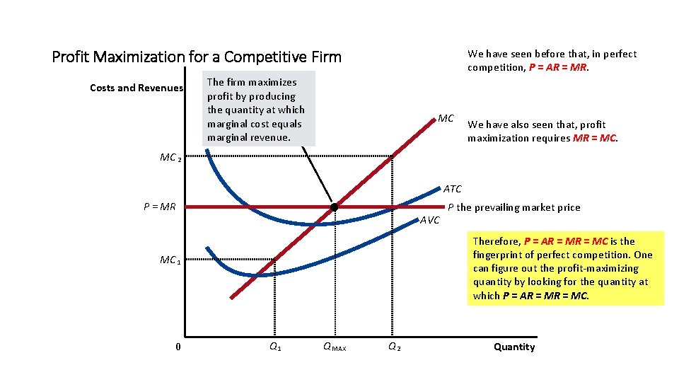
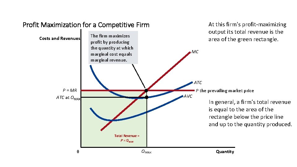
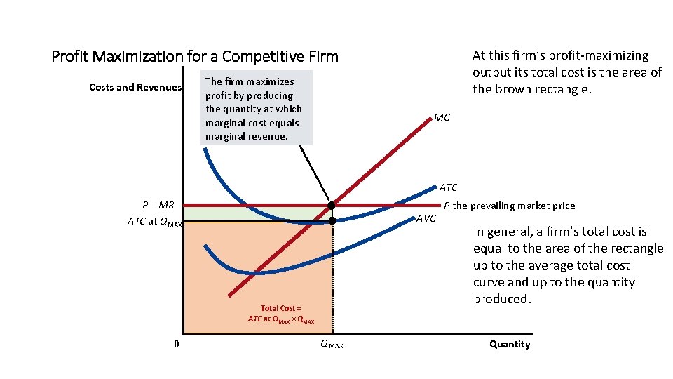
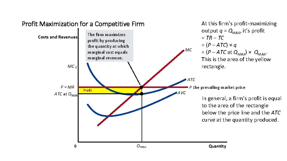
Profit Maximization for a Competitive Firm Costs and Revenues We have seen before that, in perfect competition, P = AR = MR. The firm maximizes profit by producing the quantity at which marginal cost equals marginal revenue. MC We have also seen that, profit maximization requires MR = MC. MC 2 ATC P = MR AVC Therefore, P = AR = MC is the fingerprint of perfect competition. One can figure out the profit-maximizing quantity by looking for the quantity at which P = AR = MC. MC 1 0 P the prevailing market price Q 1 Q MAX Q 2 Quantity

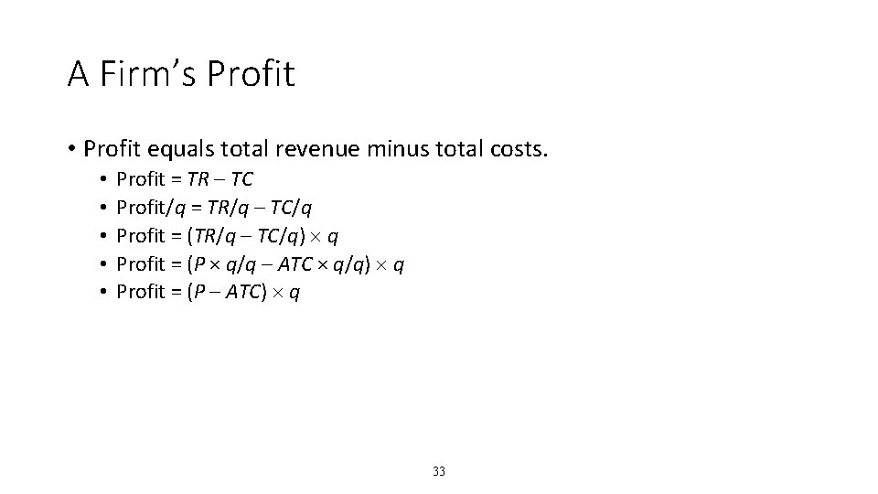
A Firm’s Profit • Profit equals total revenue minus total costs. • • • Profit = TR – TC Profit/q = TR/q – TC/q Profit = (TR/q – TC/q) q Profit = (P × q/q – ATC × q/q) q Profit = (P – ATC) q 33

Profit Maximization for a Competitive Firm Costs and Revenues The firm maximizes profit by producing the quantity at which marginal cost equals marginal revenue. At this firm’s profit-maximizing output its total revenue is the area of the green rectangle. MC ATC P = MR ATC at QMAX AVC P the prevailing market price In general, a firm’s total revenue is equal to the area of the rectangle below the price line and up to the quantity produced. Total Revenue = P × QMAX 0 Q MAX Quantity

Profit Maximization for a Competitive Firm Costs and Revenues The firm maximizes profit by producing the quantity at which marginal cost equals marginal revenue. At this firm’s profit-maximizing output its total cost is the area of the brown rectangle. MC ATC P = MR ATC at QMAX AVC Total Cost = ATC at QMAX × QMAX 0 Q MAX P the prevailing market price In general, a firm’s total cost is equal to the area of the rectangle up to the average total cost curve and up to the quantity produced. Quantity

Profit Maximization for a Competitive Firm Costs and Revenues The firm maximizes profit by producing the quantity at which marginal cost equals marginal revenue. MC MC 2 At this firm’s profit-maximizing output q = QMAX, it’s profit = TR – TC = (P – ATC) × q = (P – ATC at QMAX) × QMAX. This is the area of the yellow rectangle. ATC P = MR ATC at QMAX 0 Profit AVC Q MAX P the prevailing market price In general, a firm’s profit is equal to the area of the rectangle below the price line and the ATC curve at the quantity produced. Quantity

The Supply Curve of a Firm in a Perfectly Competitive Industry in the Short Run

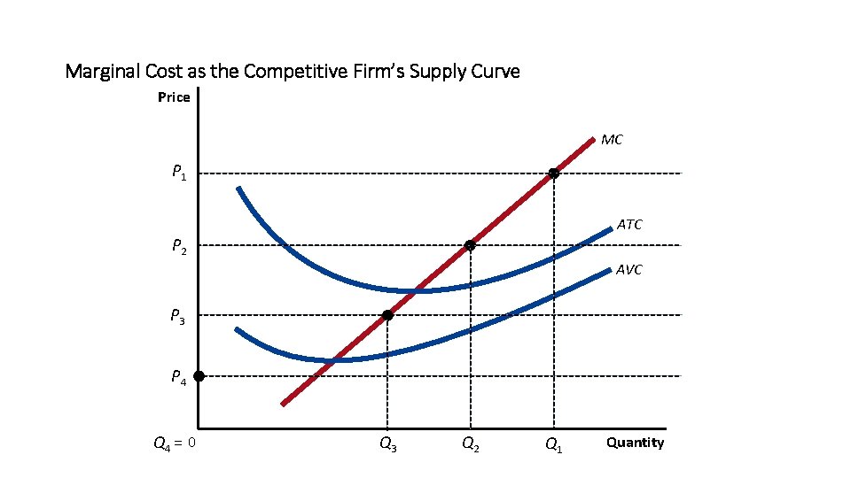
Marginal Cost as the Competitive Firm’s Supply Curve Price MC P 1 ATC P 2 AVC P 3 P 4 Q 4 = 0 Q 3 Q 2 Q 1 Quantity

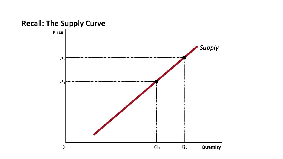
Recall: The Supply Curve Price Supply P 2 P 1 0 Q 1 Q 2 Quantity

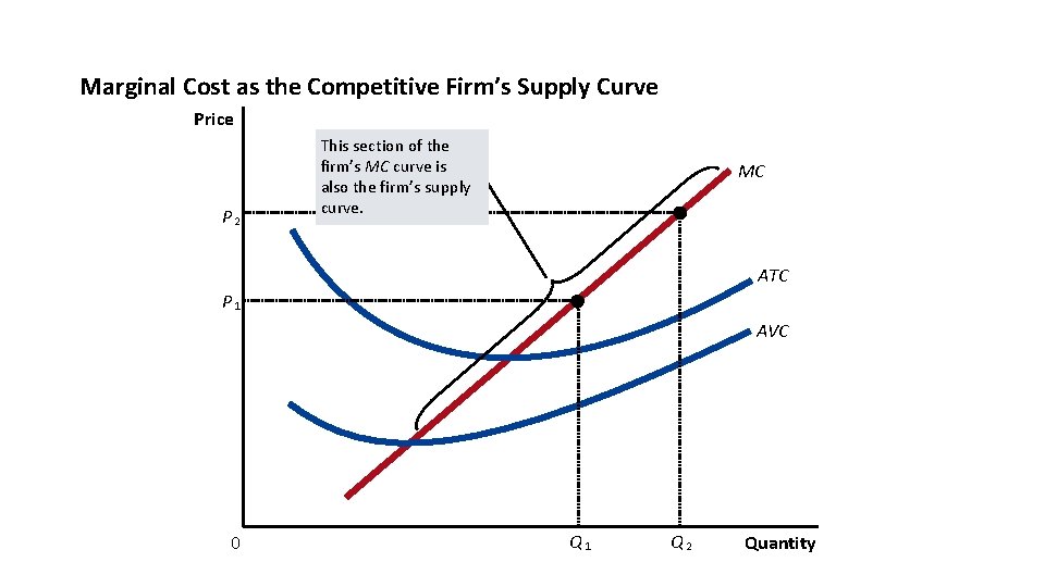
Marginal Cost as the Competitive Firm’s Supply Curve Price P 2 This section of the firm’s MC curve is also the firm’s supply curve. MC ATC P 1 AVC 0 Q 1 Q 2 Quantity

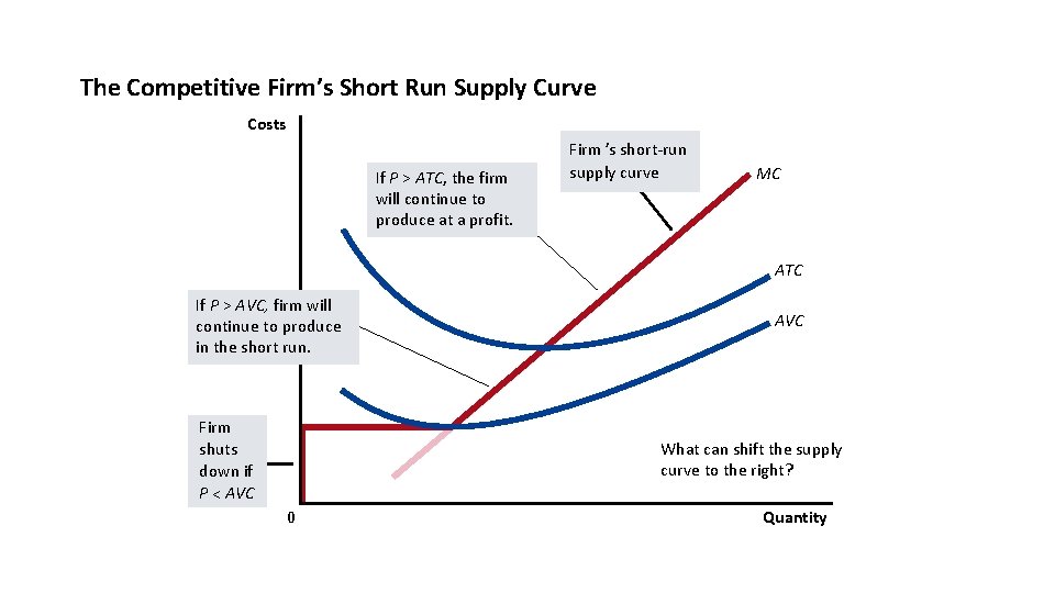
The Competitive Firm’s Short Run Supply Curve Costs If P > ATC, the firm will continue to produce at a profit. Firm ’s short-run supply curve MC ATC If P > AVC, firm will continue to produce in the short run. Firm shuts down if P < AVC What can shift the supply curve to the right? 0 Quantity

The Supply Curve of a Firm in a Perfectly Competitive Industry in the Short Run • Key idea: The Supply Curve of a firm in a perfectly competitive industry in the short run is the part of its marginal cost curve that lies above its average variable cost curve.

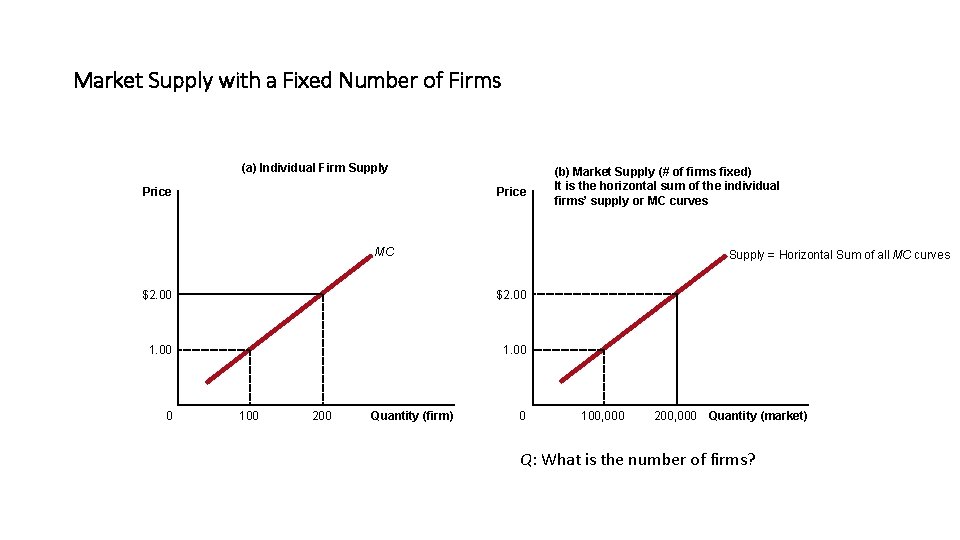
The Supply Curve of a Perfectly Competitive Industry in the Short Run • Recall that it is assumed that the number of firms is fixed in the short run • The market supply curve—or the industry supply curve or the aggregate supply curve—is the horizontal sum of the short run supply curves of the individual firms in the industry.

Market Supply with a Fixed Number of Firms (a) Individual Firm Supply Price (b) Market Supply (# of firms fixed) It is the horizontal sum of the individual firms’ supply or MC curves MC Supply = Horizontal Sum of all MC curves $2. 00 1. 00 0 100 200 Quantity (firm) 0 100, 000 200, 000 Quantity (market) Q: What is the number of firms?

Short-Run Equilibrium of a Perfectly Competitive Industry

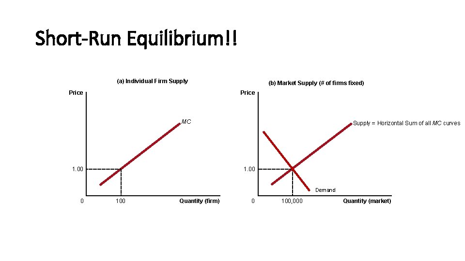
Short-Run Equilibrium!! (a) Individual Firm Supply (b) Market Supply (# of firms fixed) Price MC Supply = Horizontal Sum of all MC curves 1. 00 Demand 0 100 Quantity (firm) 0 100, 000 Quantity (market)

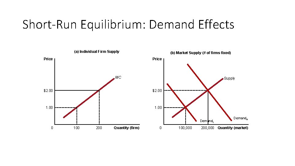
Short-Run Equilibrium: Demand Effects (a) Individual Firm Supply (b) Market Supply (# of firms fixed) Price MC Supply $2. 00 1. 00 Demand. L 0 100 200 Quantity (firm) 0 100, 000 Demand. H 200, 000 Quantity (market)

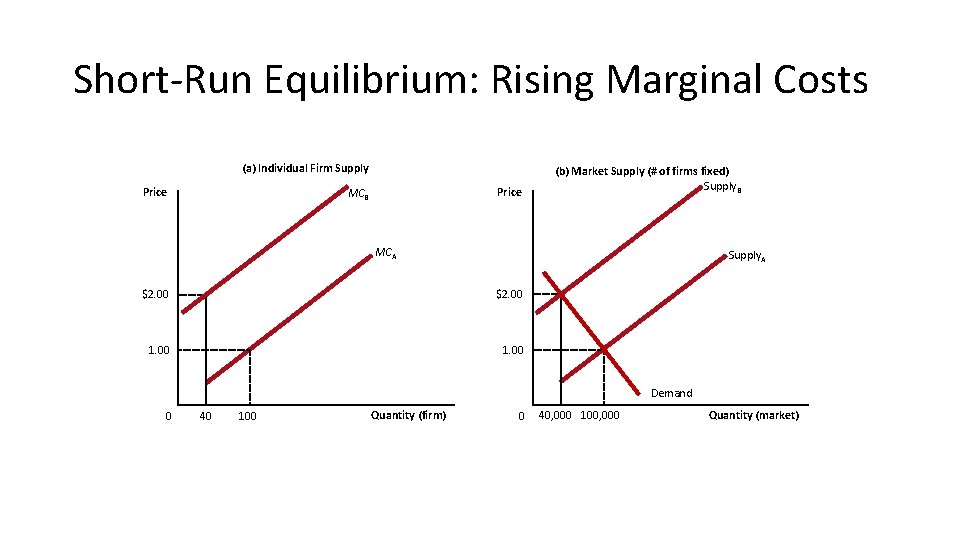
Short-Run Equilibrium: Rising Marginal Costs (a) Individual Firm Supply Price MCB (b) Market Supply (# of firms fixed) Supply. B MCA Supply. A $2. 00 1. 00 Demand 0 40 100 Quantity (firm) 0 40, 000 100, 000 Quantity (market)

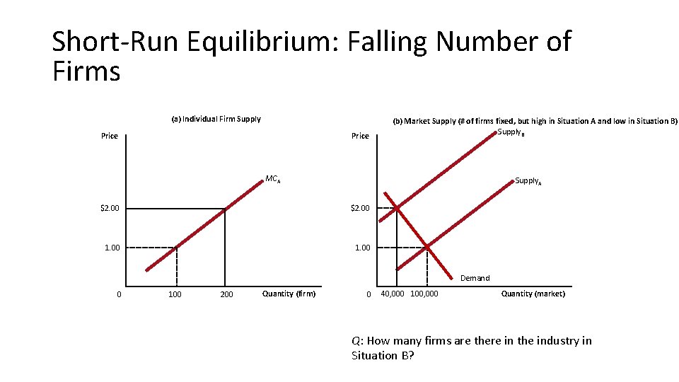
Short-Run Equilibrium: Falling Number of Firms (a) Individual Firm Supply Price (b) Market Supply (# of firms fixed, but high in Situation A and low in Situation B) Supply. B MCA Supply. A $2. 00 1. 00 Demand 0 100 200 Quantity (firm) 0 40, 000 100, 000 Quantity (market) Q: How many firms are there in the industry in Situation B?

Perfect Competition: Long Run Price = Minimum ATC; profit = zero; demand has no effect on price, and no effect on the quantity produced by a firm; demand does affect the quantity produced by the industry, and the number of firms in the industry.

Short Run and Long Run • The analysis of supply in perfect competition depends on whether it is the short run or the long run.

Short run and long run: assumptions • Key Assumption: All fixed costs are sunk costs in the short run, but not in the long run • That is, a firm does not have to pay fixed costs once it permanently leaves the industry • By contrast, a firm must keep paying its fixed costs during a temporary shutdown • Key Assumption: The number of firms in an industry is fixed in the short run, but not in the long run

Perfect Competition: Long Run Entry and Exit of Firms

The Firm’s Long-Run Decision to Exit or Enter a Market • Key assumption: In the long run, a firm will leave an industry if it sees that its profit will be negative no matter what quantity (q) it produces. • In the long run, the firm exits if it sees that its total revenue would be less than its total cost no matter what quantity (q) it might produce • That is, a firm exits if • • TR < TC, no matter what q is. TR/q < TC/q , no matter what q is. P × q/q < ATC × q/q , no matter what q is. P < ATC , no matter what q is.

The Firm’s Long-Run Decision to Exit or Enter a Market • Key assumption: A new firm will enter the industry if it expects to be profitable. • That is, a new firm will enter an industry if • • TR > TC for some value of q TR/q > TC/q for some value of q P × q/q > ATC × q/q , for some value of q P > ATC for some value of q

Perfect Competition: Long Run The Market Price and the Quantity Produced by Each Firm

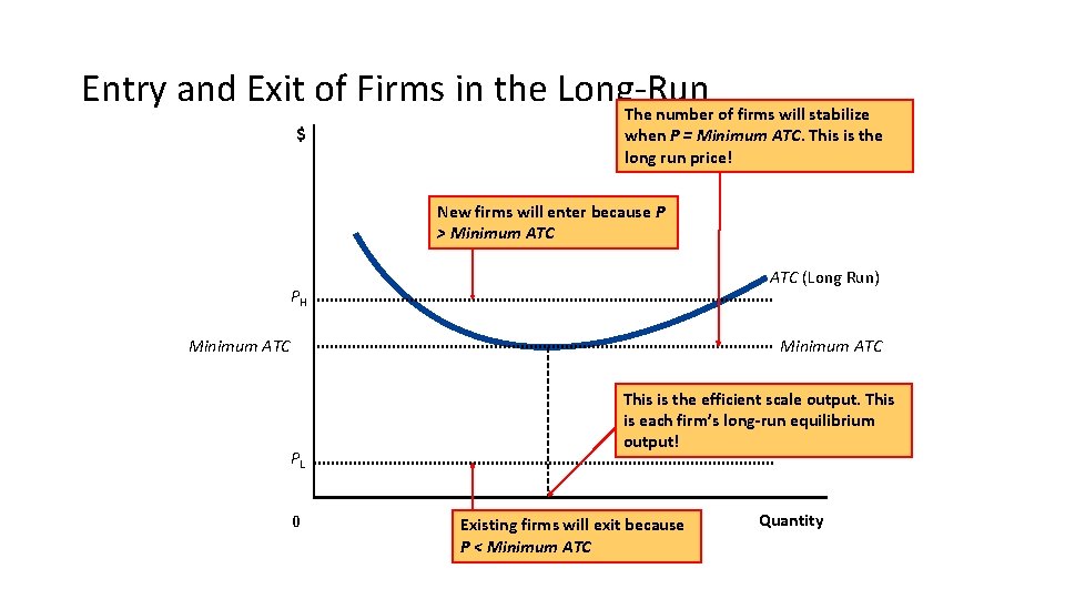
Long-Run Equilibrium • Key definition: An industry is in long-run equilibrium if the number of firms is constant even though entry and exit are both possible • Key idea: This means firms earn zero profits in the long-run equilibrium in perfect competition • Had firms earned positive profits, new firms would’ve entered. This would’ve driven prices down till profits reached zero. • Had firms’ profits been negative, they would’ve begun to leave. This would’ve driven prices up till profits again reached zero.

Entry and Exit of Firms in the Long-Run The number of firms will stabilize $ when P = Minimum ATC. This is the long run price! New firms will enter because P > Minimum ATC (Long Run) PH Minimum ATC PL 0 This is the efficient scale output. This is each firm’s long-run equilibrium output! Existing firms will exit because P < Minimum ATC Quantity

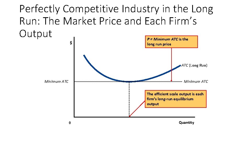
Perfectly Competitive Industry in the Long Run: The Market Price and Each Firm’s Output $ P = Minimum ATC is the long run price ATC (Long Run) Minimum ATC The efficient scale output is each firm’s long-run equilibrium output 0 Quantity

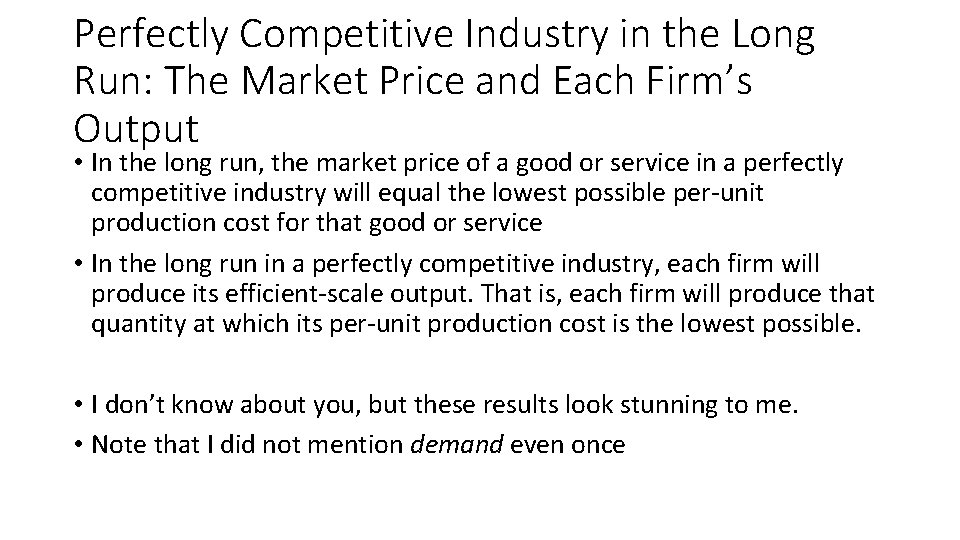
Perfectly Competitive Industry in the Long Run: The Market Price and Each Firm’s Output • In the long run, the market price of a good or service in a perfectly competitive industry will equal the lowest possible per-unit production cost for that good or service • In the long run in a perfectly competitive industry, each firm will produce its efficient-scale output. That is, each firm will produce that quantity at which its per-unit production cost is the lowest possible. • I don’t know about you, but these results look stunning to me. • Note that I did not mention demand even once

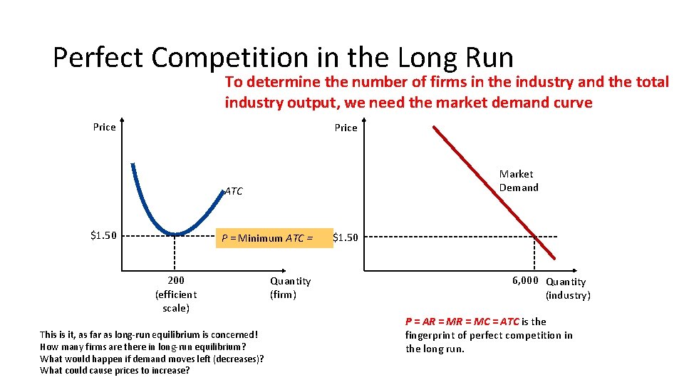
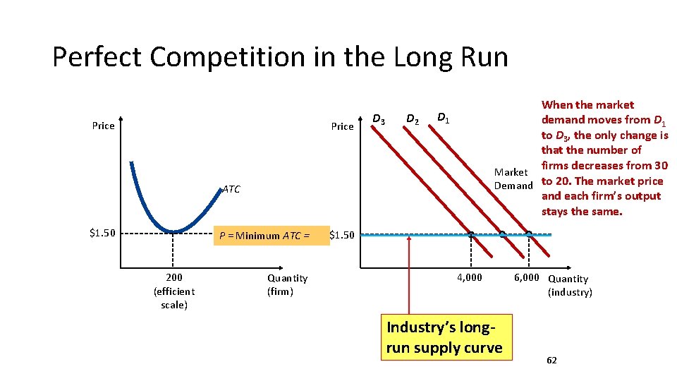
Perfect Competition in the Long Run To determine the number of firms in the industry and the total industry output, we need the market demand curve Price Market Demand ATC $1. 50 P = Minimum ATC = 200 (efficient scale) This is it, as far as long-run equilibrium is concerned! How many firms are there in long-run equilibrium? What would happen if demand moves left (decreases)? What could cause prices to increase? Quantity (firm) $1. 50 6, 000 Quantity (industry) P = AR = MC = ATC is the fingerprint of perfect competition in the long run.

Perfect Competition in the Long Run Price D 3 D 2 When the market demand moves from D 1 to D 3, the only change is that the number of firms decreases from 30 Market Demand to 20. The market price and each firm’s output stays the same. D 1 ATC $1. 50 P = Minimum ATC = 200 (efficient scale) Quantity (firm) $1. 50 4, 000 Industry’s longrun supply curve 6, 000 Quantity (industry) 62

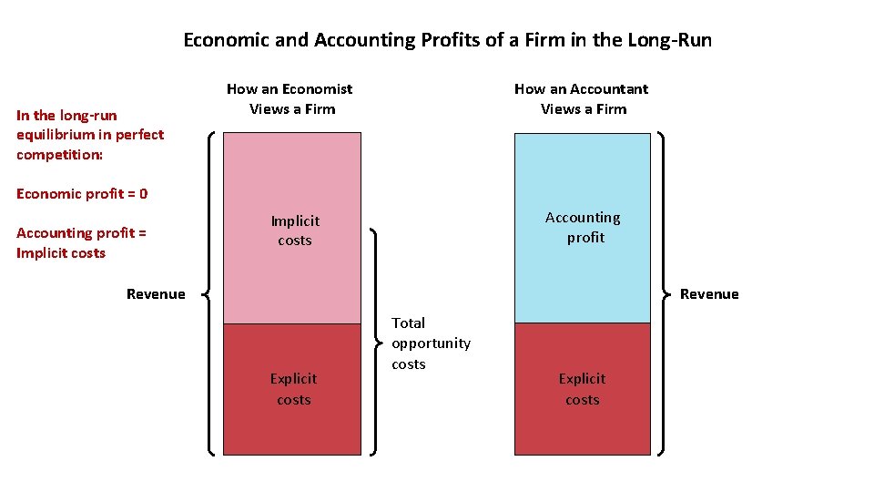
Perfect Competition: Long Run How can profits be zero? We saw earlier that each firm earns zero profits in long-run equilibrium in perfect competition. How can that be? (Hint: It has to do with the distinction between accounting profit and economic profit. )

Why Do Competitive Firms Stay in Business If They Make Zero Profit? • Profit = TR – TC • Total cost = explicit cost + implicit cost. • Explicit cost is the market value of resources a firm buys from others • Implicit cost is the market value of resources given for free to the firm (usually by the firm’s owners) • Profit = 0 implies TR = explicit cost + implicit cost • So, in the long-run zero-profit equilibrium, the firm earns enough revenue to pay its bills and also compensate the owners for the resources they provide to keep the business going. • So, don’t feel sorry for the owners!

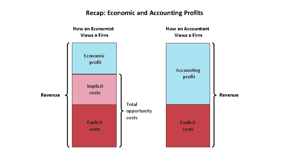
Recap: Economic and Accounting Profits How an Economist Views a Firm How an Accountant Views a Firm Economic profit Accounting profit Revenue Implicit costs Explicit costs Revenue Total opportunity costs Explicit costs

Economic and Accounting Profits of a Firm in the Long-Run In the long-run equilibrium in perfect competition: How an Economist Views a Firm How an Accountant Views a Firm Economic profit = 0 Accounting profit = Implicit costs Accounting profit Implicit costs Revenue Explicit costs Total opportunity costs Explicit costs

Combining short-run and longrun analysis We will now work through what happens when the demand for a product increases.

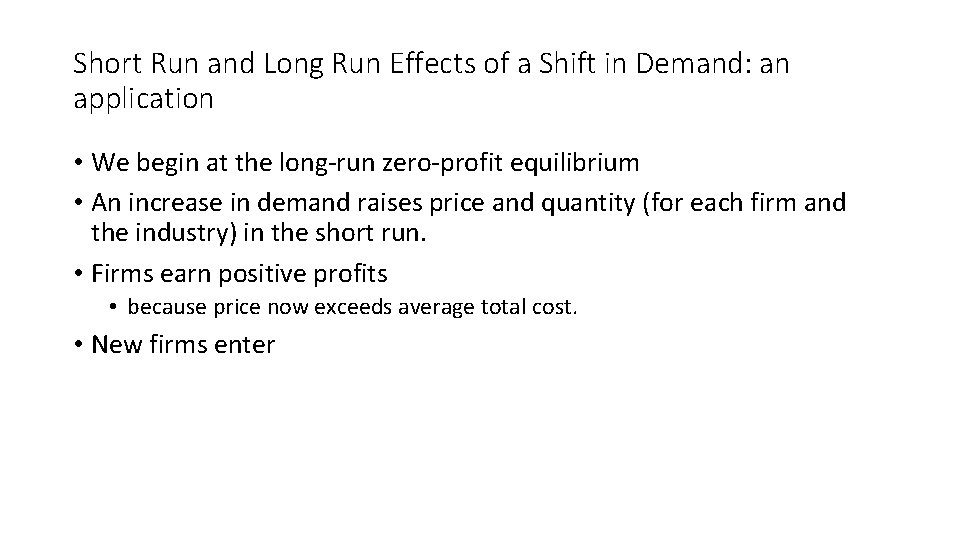
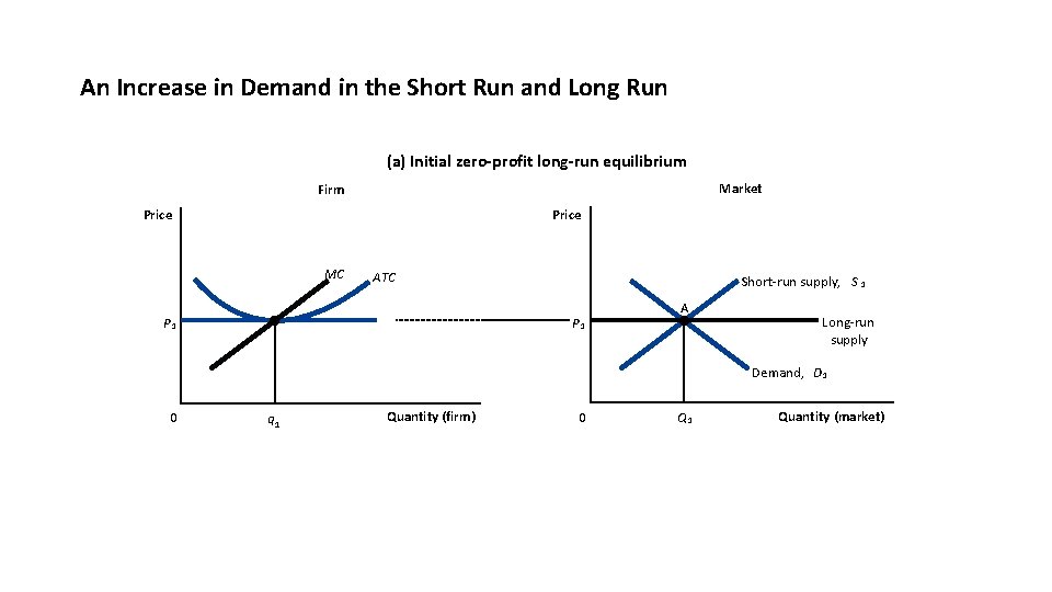
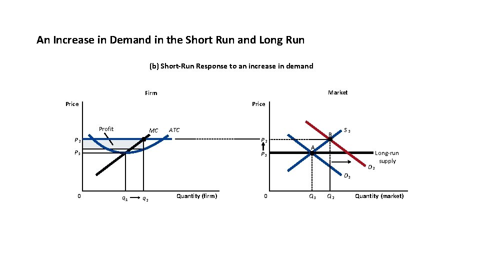
Short Run and Long Run Effects of a Shift in Demand: an application • We begin at the long-run zero-profit equilibrium • An increase in demand raises price and quantity (for each firm and the industry) in the short run. • Firms earn positive profits • because price now exceeds average total cost. • New firms enter

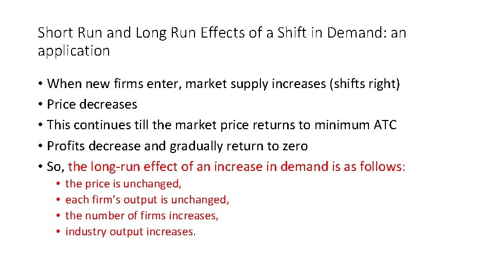
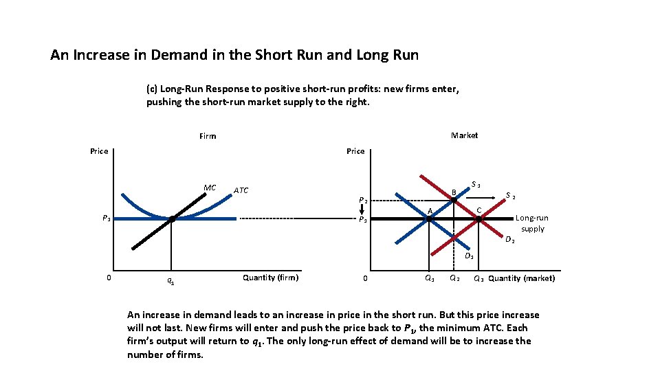
Short Run and Long Run Effects of a Shift in Demand: an application • When new firms enter, market supply increases (shifts right) • Price decreases • This continues till the market price returns to minimum ATC • Profits decrease and gradually return to zero • So, the long-run effect of an increase in demand is as follows: • • the price is unchanged, each firm’s output is unchanged, the number of firms increases, industry output increases.

An Increase in Demand in the Short Run and Long Run (a) Initial zero-profit long-run equilibrium Market Firm Price MC ATC Short-run supply, S 1 P 1 A Long-run supply Demand, D 1 0 q 1 Quantity (firm) 0 Q 1 Quantity (market)

An Increase in Demand in the Short Run and Long Run (b) Short-Run Response to an increase in demand Market Firm Price Profit MC ATC P 2 P 1 B S 1 A D 2 Long-run supply D 1 0 q 1 q 2 Quantity (firm) 0 Q 1 Q 2 Quantity (market)

An Increase in Demand in the Short Run and Long Run (c) Long-Run Response to positive short-run profits: new firms enter, pushing the short-run market supply to the right. Market Firm Price MC ATC P 1 P 2 P 1 B S 1 S 2 C A D 2 Long-run supply D 1 0 q 1 Quantity (firm) 0 Q 1 Q 2 Q 3 Quantity (market) An increase in demand leads to an increase in price in the short run. But this price increase will not last. New firms will enter and push the price back to P 1, the minimum ATC. Each firm’s output will return to q 1. The only long-run effect of demand will be to increase the number of firms.

Any Questions?