Path Models for Time Series Anomaly Detection Matt

Path Models for Time Series Anomaly Detection Matt Mahoney

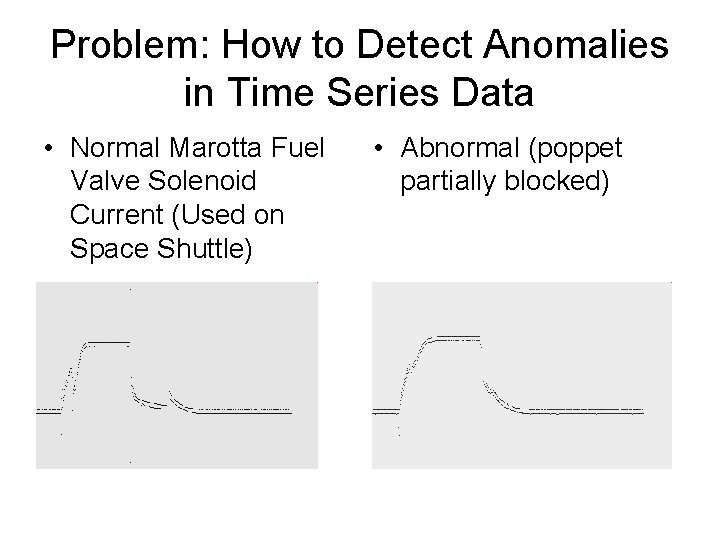
Problem: How to Detect Anomalies in Time Series Data • Normal Marotta Fuel Valve Solenoid Current (Used on Space Shuttle) • Abnormal (poppet partially blocked)

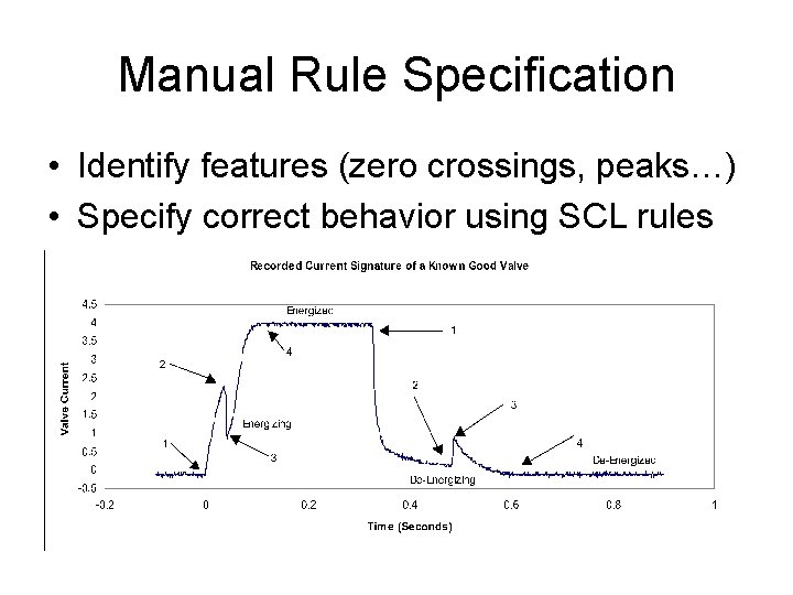
Manual Rule Specification • Identify features (zero crossings, peaks…) • Specify correct behavior using SCL rules

Automatic Rule Generation (Stan Salvador) • Segment training data (GECKO) • Rule induction (RIPPER) to map data points to segments • Create linear state machine table in SCL

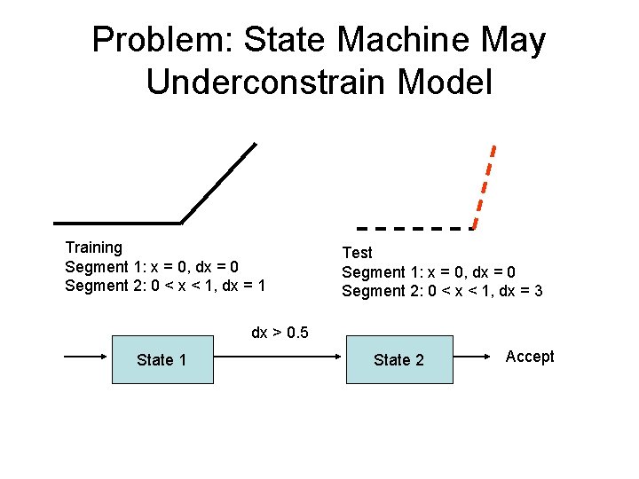
Problem: State Machine May Underconstrain Model Training Segment 1: x = 0, dx = 0 Segment 2: 0 < x < 1, dx = 1 Test Segment 1: x = 0, dx = 0 Segment 2: 0 < x < 1, dx = 3 dx > 0. 5 State 1 State 2 Accept

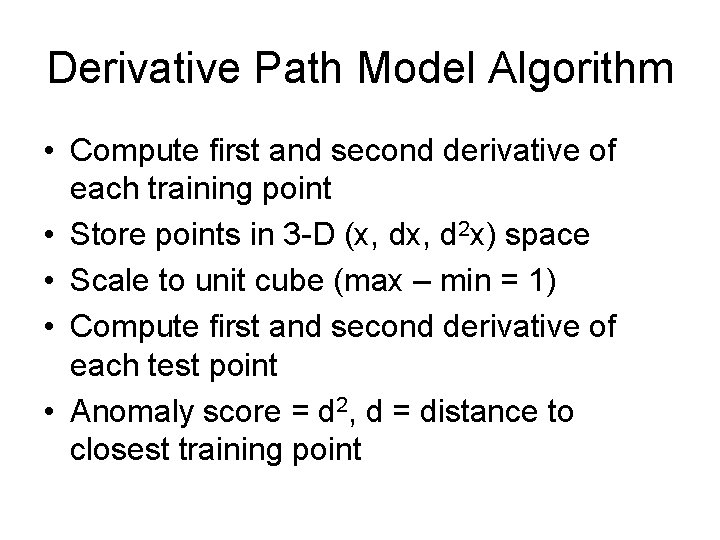
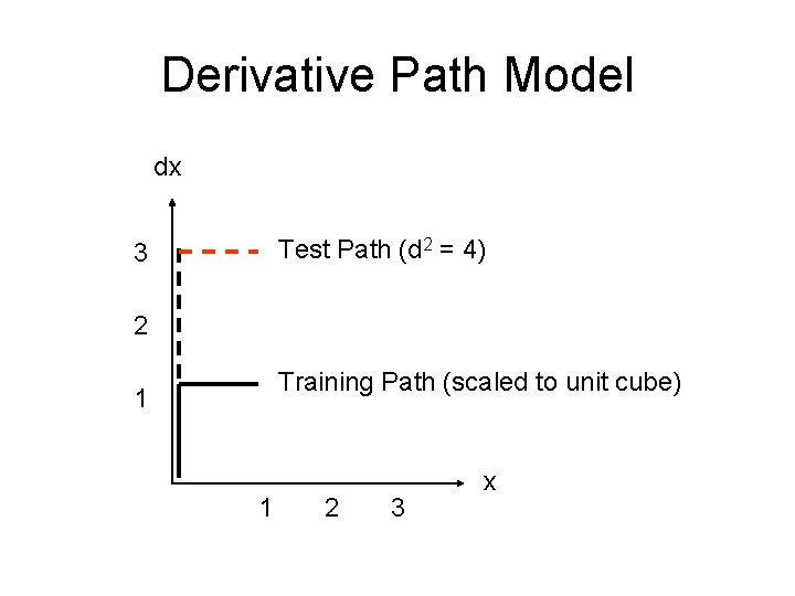
Derivative Path Model Algorithm • Compute first and second derivative of each training point • Store points in 3 -D (x, d 2 x) space • Scale to unit cube (max – min = 1) • Compute first and second derivative of each test point • Anomaly score = d 2, d = distance to closest training point

Derivative Path Model dx Test Path (d 2 = 4) 3 2 Training Path (scaled to unit cube) 1 1 2 3 x

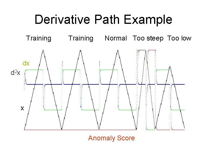
Derivative Path Example Training Normal Too steep Too low dx d 2 x x Anomaly Score

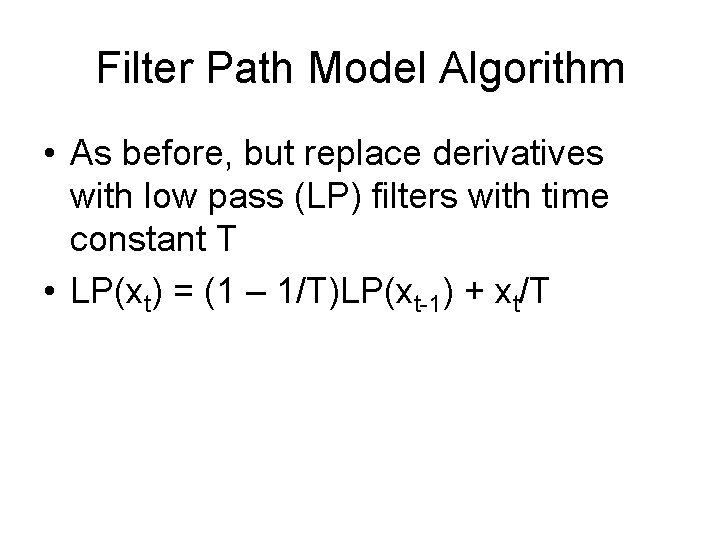
Filter Path Model Algorithm • As before, but replace derivatives with low pass (LP) filters with time constant T • LP(xt) = (1 – 1/T)LP(xt-1) + xt/T

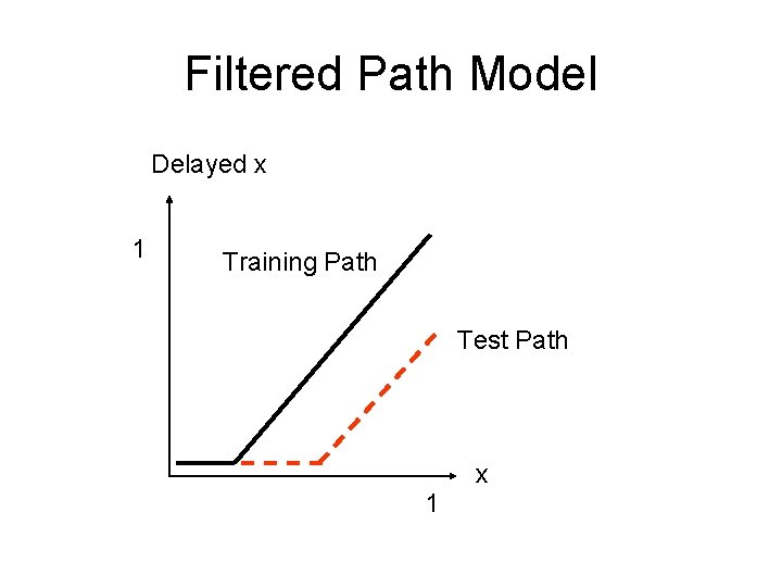
Filtered Path Model Delayed x 1 Training Path Test Path x 1

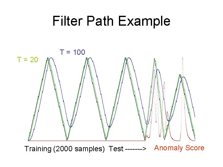
Filter Path Example T = 20 T = 100 Training (2000 samples) Test -------> Anomaly Score

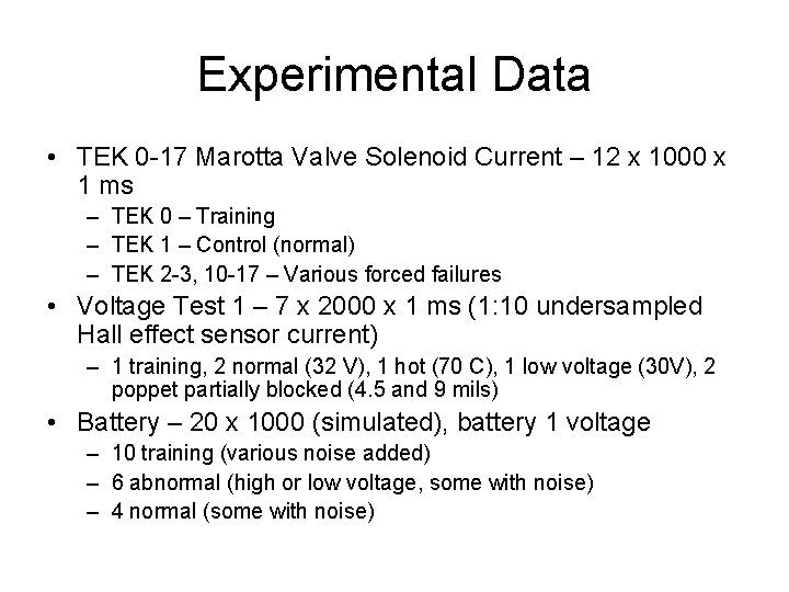
Experimental Data • TEK 0 -17 Marotta Valve Solenoid Current – 12 x 1000 x 1 ms – TEK 0 – Training – TEK 1 – Control (normal) – TEK 2 -3, 10 -17 – Various forced failures • Voltage Test 1 – 7 x 2000 x 1 ms (1: 10 undersampled Hall effect sensor current) – 1 training, 2 normal (32 V), 1 hot (70 C), 1 low voltage (30 V), 2 poppet partially blocked (4. 5 and 9 mils) • Battery – 20 x 1000 (simulated), battery 1 voltage – 10 training (various noise added) – 6 abnormal (high or low voltage, some with noise) – 4 normal (some with noise)

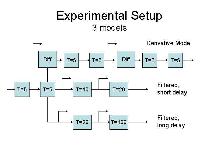
Experimental Setup 3 models Derivative Model Diff T=5 T=5 T=10 T=20 T=5 Diff T=5 T=20 Filtered, short delay T=100 Filtered, long delay

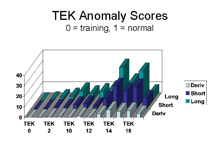
TEK Anomaly Scores 0 = training, 1 = normal

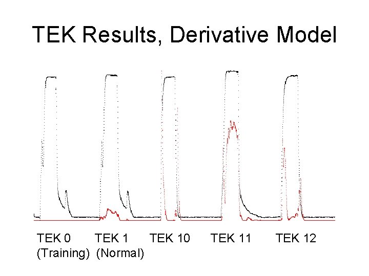
TEK Results, Derivative Model TEK 0 TEK 10 (Training) (Normal) TEK 11 TEK 12

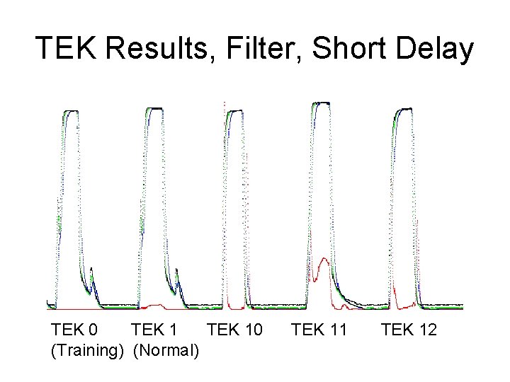
TEK Results, Filter, Short Delay TEK 0 TEK 10 (Training) (Normal) TEK 11 TEK 12

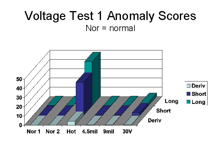
Voltage Test 1 Anomaly Scores Nor = normal

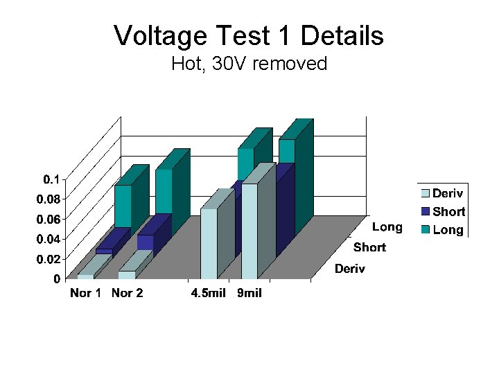
Voltage Test 1 Details Hot, 30 V removed

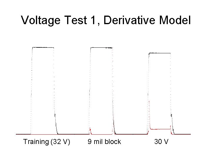
Voltage Test 1, Derivative Model Training (32 V) 9 mil block 30 V

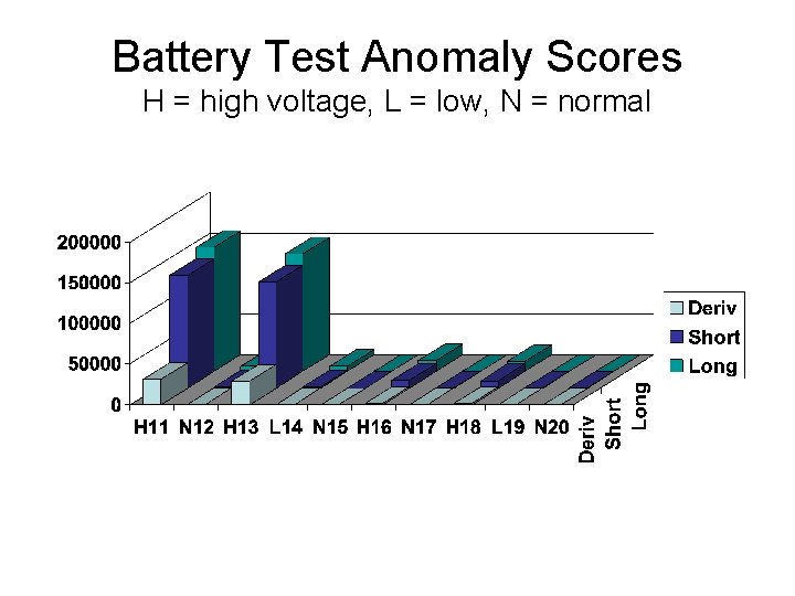
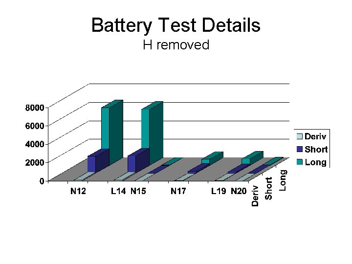
Battery Test Anomaly Scores H = high voltage, L = low, N = normal

Battery Test Details H removed

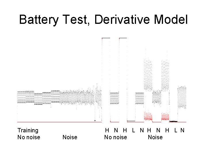
Battery Test, Derivative Model Training No noise Noise H N H L N No noise Noise

Summary • Path modeling compares test point features to training data – Features may be derivatives or filtered data • Numeric anomaly score (user threshold) • Constrains all data in all directions • Straightforward extension to more dimensions (either features or inputs)

Limitations • No long term state – But filters provide a short term state • No concise (SCL) representation – Point set could have piecewise polynomial approximation • O(n 2) test speed – Must compare each test point with all training points – Could be faster with piecewise model • Does not generalize to unseen data – Considers all dimensions equally important

Future Work • Replace point list with piecewise linear model – Segment path with Gecko or similar – SCL function to compute distance • Extend to multiple dimensions/features – Variable delay filters to add state – May worsen generalization, too many irrelevant dimensions • “Tube” model to improve generalization – Initial training data defines path – Additional training stretches tube (scaling matrix) around path to fit

More information • Open source implementation of path modeling (tsad 1. cpp, tsad 3. cpp) • Technical report of this presentation • http: //cs. fit. edu/~mmahoney/nasa/