Optimal Preventative Maintenance Scheduling in Process Plants La

Optimal Preventative Maintenance Scheduling in Process Plants La. Risa Sergent Jeff Sorenson University of Oklahoma School of Chemical, Biological, and Materials Engineering April 29 th, 2008

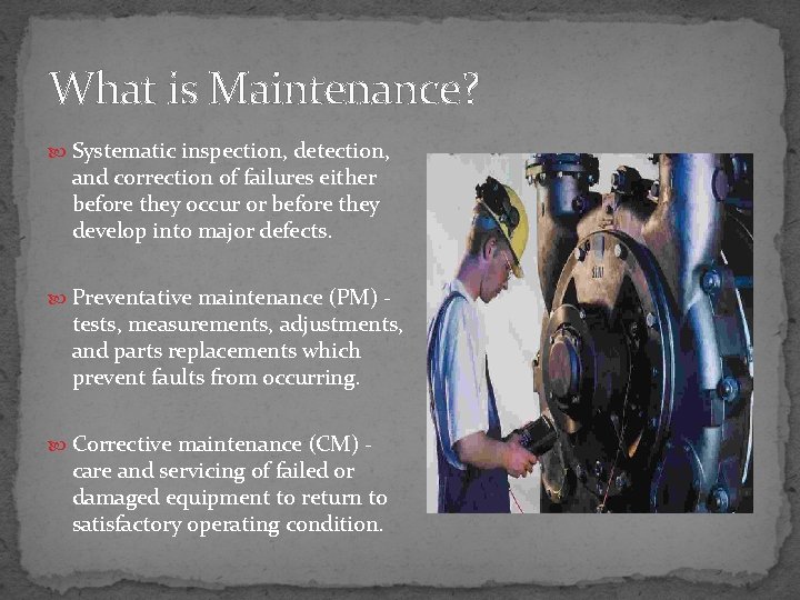
What is Maintenance? Systematic inspection, detection, and correction of failures either before they occur or before they develop into major defects. Preventative maintenance (PM) - tests, measurements, adjustments, and parts replacements which prevent faults from occurring. Corrective maintenance (CM) - care and servicing of failed or damaged equipment to return to satisfactory operating condition.

Modern Maintenance Philosophy �Favors constant preventative maintenance. �Economic trade-offs � Cost of labor � Loss of product � Replacement costs � Downtime for PM �How much preventative maintenance is economically optimal? � 30%-50% of a plant’s operating budget �Goals of maintenance scheduling � maximize safety � minimize total cost

Our Model Parameters to be manipulated Spare parts policy Frequency of preventative maintenance Labor resources Objective function to be minimized: Total maintenance costs (PM + CM) Total economic loss

Assumptions in the Model PM takes place on regular intervals (fraction of MTBF) Time to complete diagnosis of failure negligible All workers perform every maintenance task Equipment failures prioritized by severity Emergencies take precedence over scheduled maintenance Parts not on hand arrive in no more than a week Repaired equipment is deemed as good as new

Monte Carlo Simulation Samples failure rate of the equipment and the probability of each failure mode (i. e. electrical, mechanical, etc. ) Associated cost of each failure is calculated Man hours are assigned first to each needed CM, then to scheduled PM When the man hours for the week are expended, no more maintenance takes place Average total cost is determined for a large number of samples (10, 000)

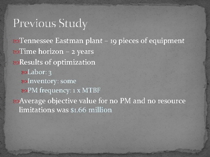
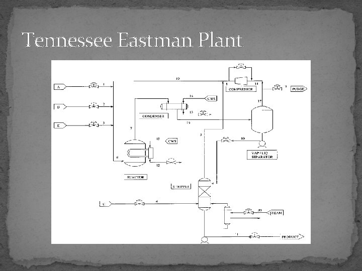
Previous Study Tennessee Eastman plant – 19 pieces of equipment Time horizon – 2 years Results of optimization Labor: 3 Inventory: some PM frequency: 1 x MTBF Average objective value for no PM and no resource limitations was $1. 66 million

Tennessee Eastman Plant

Additions to the previous model Risk analysis Total cost versus probability of incidence Consider Value at Risk in addition to Average Total Cost Model applied to larger process New values determined for: Optimal labor force Optimal PM interval Genetic algorithm applied to larger process All variables manipulated simultaneously

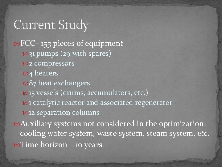
Current Study FCC– 153 pieces of equipment 31 pumps (29 with spares) 2 compressors 4 heaters 87 heat exchangers 15 vessels (drums, accumulators, etc. ) 1 catalytic reactor and associated regenerator 12 separation columns Auxiliary systems not considered in the optimization: cooling water system, waste system, steam system, etc. Time horizon – 10 years

Assumptions Specific to the FCC Pumps Those with spares do not incur economic loss upon failing. PM is done on spare following CM on main pump, and the cost is included in the CM cost. The TNCM includes time for PM on the spare. Columns Two main columns – if one fails, the other begins running at max capacity.

Assumptions Specific to the FCC Vessels and tanks Failure results in loss of throughput for that tank only; rest of the product throughput is not lost. Heat exchangers Failure reduces efficiency of the process. Being repaired HE can be bypassed. Bypassed HE causes loss in product relative to the portion of heat duty lost. Reactors and compressors Failure results in total throughput lost.

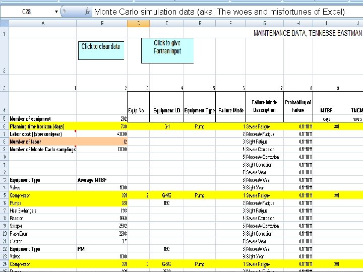
Monte Carlo simulation data (aka. The woes and misfortunes of Excel)

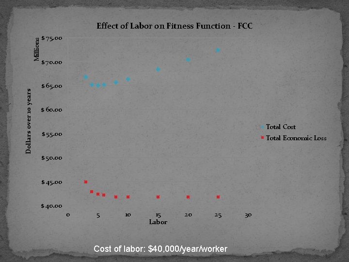
Dollars over 10 years Millions Effect of Labor on Fitness Function - FCC $ 75. 00 $ 70. 00 $ 65. 00 $ 60. 00 Total Cost $ 55. 00 Total Economic Loss $ 50. 00 $ 45. 00 $ 40. 00 0 5 10 15 Labor 20 25 Cost of labor: $40, 000/year/worker 30

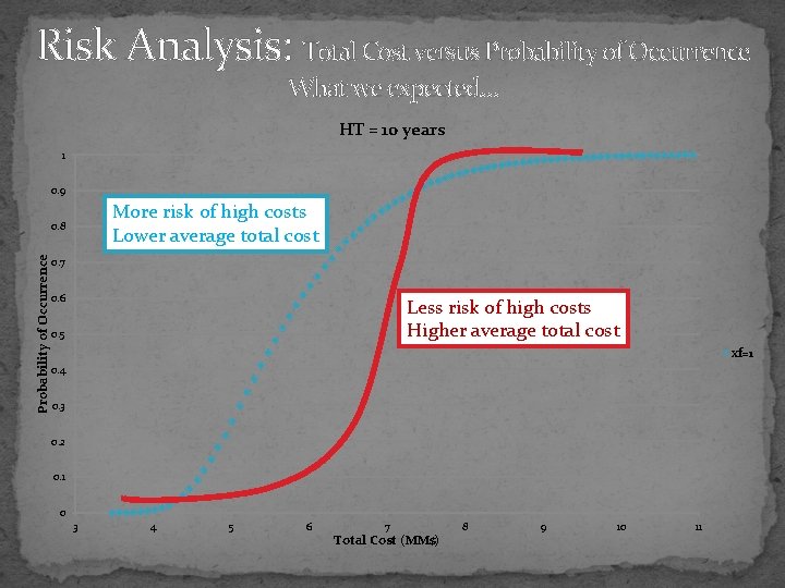
Risk Analysis: Total Cost versus Probability of Occurrence What we expected… HT = 10 years 1 0. 9 More risk of high costs Lower average total cost Probability of Occurrence 0. 8 0. 7 0. 6 Less risk of high costs Higher average total cost 0. 5 xf=1 0. 4 0. 3 0. 2 0. 1 0 3 4 5 6 7 Total Cost (MM$) 8 9 10 11

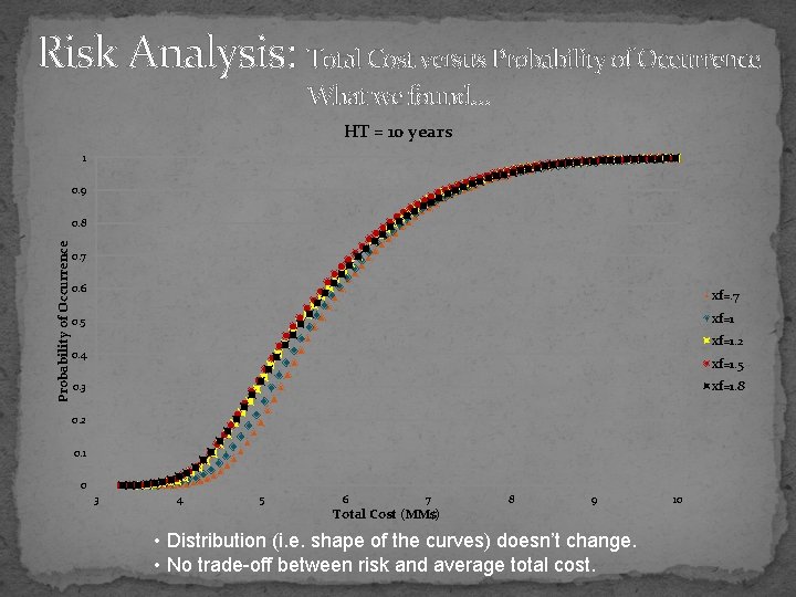
Risk Analysis: Total Cost versus Probability of Occurrence What we found… HT = 10 years 1 0. 9 Probability of Occurrence 0. 8 0. 7 0. 6 xf=. 7 xf=1 0. 5 xf=1. 2 0. 4 xf=1. 5 xf=1. 8 0. 3 0. 2 0. 1 0 3 4 5 6 7 Total Cost (MM$) 8 9 • Distribution (i. e. shape of the curves) doesn’t change. • No trade-off between risk and average total cost. 10

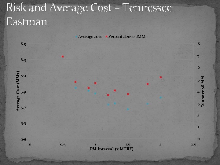
Risk and Average Cost – Tennessee Eastman Average cost Percent above 8 MM 6. 5 8 7 6. 3 6. 1 5 5. 9 4 3 5. 7 2 5. 5 1 5. 3 0 0 0. 5 1 1. 5 PM Interval (x MTBF) 2 2. 5 % above $8 MM Average Cost (MM$) 6

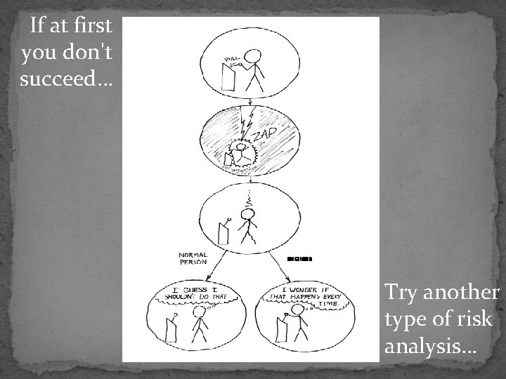
If at first you don't succeed… ENGINEER Try another type of risk analysis…

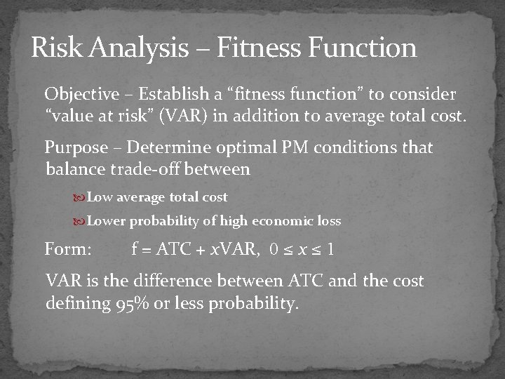
Risk Analysis – Fitness Function Objective – Establish a “fitness function” to consider “value at risk” (VAR) in addition to average total cost. Purpose – Determine optimal PM conditions that balance trade-off between Low average total cost Lower probability of high economic loss Form: f = ATC + x. VAR, 0 ≤ x ≤ 1 VAR is the difference between ATC and the cost defining 95% or less probability.

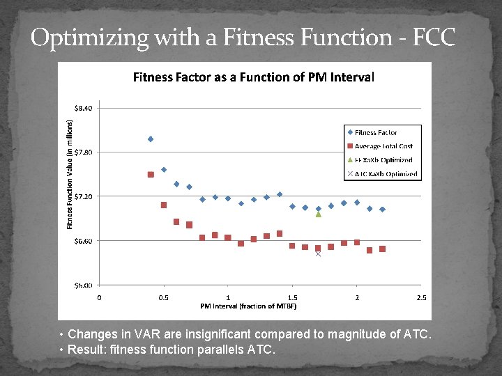
Optimizing with a Fitness Function - FCC • Changes in VAR are insignificant compared to magnitude of ATC. • Result: fitness function parallels ATC.

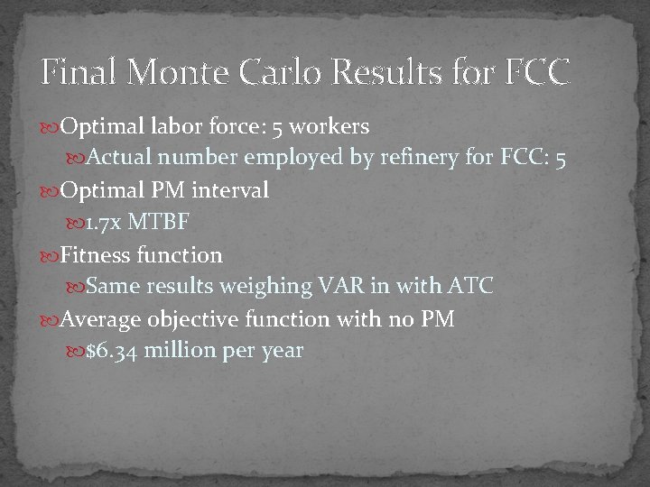
Final Monte Carlo Results for FCC Optimal labor force: 5 workers Actual number employed by refinery for FCC: 5 Optimal PM interval 1. 7 x MTBF Fitness function Same results weighing VAR in with ATC Average objective function with no PM $6. 34 million per year

PM Optimization by Component Evaluate a specific component at varied PM interval by simulations with all other PM schedules constant. Determine optimal PM frequency for the chosen component. Lower average cost Lower probability of high economic loss Run “optimized” simulation using optimal value for each specific component. Compare values of economic loss to those obtained using a single “x-factor” to vary overall PM frequency.

Genetic Algorithms Evaluates multiple variables simultaneously. Each variable becomes a “gene” on the maintenance model “chromosome. ” A population of chromosomes is randomly generated. Each chromosome (model) is evaluated to determine its “fitness” in comparison to others in the population. More “fit” chromosomes more likely to reproduce and continue to exist in new generations. Crossover and mutation exist.

Genetic Algorithms “Parents” chosen randomly from reproduction pool Offspring are identical to parents UNLESS Crossover occurs: offspring “swap” one gene. (random) Mutation occurs: offspring has one gene (random) replaced with a new value. Crossover and mutation prevent premature convergence Reduce likelihood of optimizing to a “local minimum. ” Fitness of parents and offspring evaluated. “Best” chromosome automatically enters new generation

Genetic Algorithms Operation of Genetic Algorithm Define range of values for parameter generation. PM intervals set between 0. 5 and 1. 6 for non-interfering pieces of equipment. PM intervals set between 0. 3 and 1. 1 for interfering pieces of equipment. Specify population size, crossover probability, mutation probability, and number of generations. Complication: Each generation takes 48 -65 minutes to evaluate. Running the algorithm literally takes days.

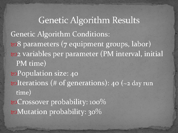
Genetic Algorithm Results Genetic Algorithm Conditions: 8 parameters (7 equipment groups, labor) 2 variables per parameter (PM interval, initial PM time) Population size: 40 Iterations (# of generations): 40 (~2 day run time) Crossover probability: 100% Mutation probability: 30%

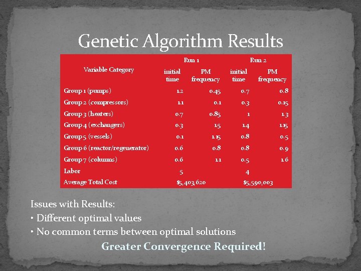
Genetic Algorithm Results Run 1 Variable Category initial time Run 2 PM frequency initial time PM frequency Group 1 (pumps) 1. 2 0. 45 0. 7 0. 8 Group 2 (compressors) 1. 1 0. 3 0. 15 Group 3 (heaters) 0. 7 0. 85 1 1. 3 Group 4 (exchangers) 0. 3 1. 5 1. 4 1. 15 Group 5 (vessels) 0. 1 1. 15 0. 8 0. 5 Group 6 (reactor/regenerator) 0. 6 0. 8 0. 9 Group 7 (columns) 0. 6 1. 1 0. 5 1. 6 Labor 5 Average Total Cost $5, 403, 620 4 $5, 590, 003 Issues with Results: • Different optimal values • No common terms between optimal solutions Greater Convergence Required!

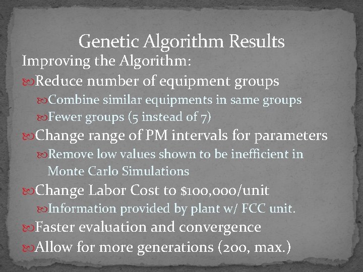
Genetic Algorithm Results Improving the Algorithm: Reduce number of equipment groups Combine similar equipments in same groups Fewer groups (5 instead of 7) Change range of PM intervals for parameters Remove low values shown to be inefficient in Monte Carlo Simulations Change Labor Cost to $100, 000/unit Information provided by plant w/ FCC unit. Faster evaluation and convergence Allow for more generations (200, max. )

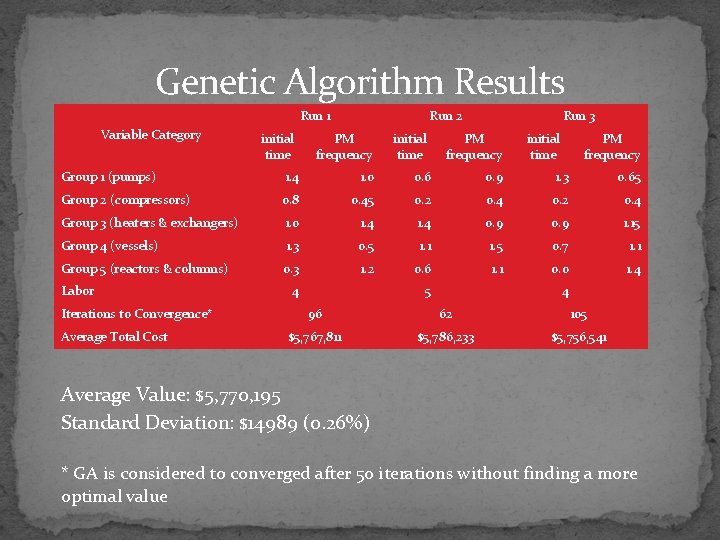
Genetic Algorithm Results Run 1 Variable Category initial time Run 2 PM frequency initial time Run 3 PM frequency initial time PM frequency Group 1 (pumps) 1. 4 1. 0 0. 6 0. 9 1. 3 0. 65 Group 2 (compressors) 0. 8 0. 45 0. 2 0. 4 Group 3 (heaters & exchangers) 1. 0 1. 4 0. 9 1. 15 Group 4 (vessels) 1. 3 0. 5 1. 1 1. 5 0. 7 1. 1 Group 5 (reactors & columns) 0. 3 1. 2 0. 6 1. 1 0. 0 1. 4 Labor Iterations to Convergence* Average Total Cost 4 5 4 96 62 105 $5, 767, 811 $5, 786, 233 $5, 756, 541 Average Value: $5, 770, 195 Standard Deviation: $14989 (0. 26%) * GA is considered to converged after 50 iterations without finding a more optimal value

Genetic Algorithm: Further Work Separate equipment groups for more optimal PM interval of each component. Longer computation time required for each generation Slower convergence to optimal PM policy Modify mutation and crossover probability to reduce risk of local minimums being found as optimal solutions. More generations required for convergence to optimal policy Refine data used in analysis More accurate, process-specific data will increase value of PM solutions obtained by algorithm.

La. Risa Sergent Jeff Sorenson Optimal Preventative Maintenance Scheduling in Process Plants Thank you.