Nonnegative Matrix Factorization with Sparseness Constraints Patrik O

Non-negative Matrix Factorization with Sparseness Constraints Patrik O. Hoyer Journal of Machine Learning Research (2004) Presenter : 張庭豪

Outline Introduction Non-negative Matrix Factorization Adding Sparseness Constraints to NMF Experiments with Sparseness Constraints Conclusions 2

Introduction A fundamental problem in many data-analysis tasks is to find a suitable representation of the data. A useful representation typically makes latent structure in the data explicit, and often reduces the dimensionality of the data so that further computational methods can be applied. Non-negative matrix factorization (NMF) is a recent method for finding such a representation. The non-negativity constraints make the representation purely additive (allowing no subtractions). 3

Introduction However, because the sparseness given by NMF is somewhat of a side-effect rather than a goal, one cannot in any way control the degree to which the representation is sparse. In many applications, more direct control over the properties of the representation is needed. In this paper, we extend NMF to include the option to control sparseness explicitly. We show that this allows us to discover parts-based representations that are qualitatively better than those given by basic NMF. 4

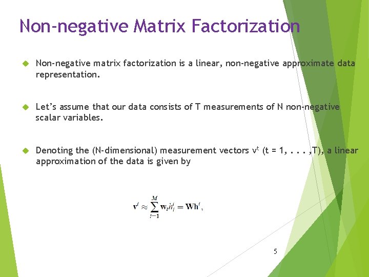
Non-negative Matrix Factorization Non-negative matrix factorization is a linear, non-negative approximate data representation. Let’s assume that our data consists of T measurements of N non-negative scalar variables. Denoting the (N-dimensional) measurement vectors vt (t = 1, . . . , T), a linear approximation of the data is given by 5

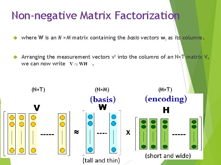
Non-negative Matrix Factorization where W is an N ×M matrix containing the basis vectors wi as its columns. Arranging the measurement vectors vt into the columns of an N×T matrix V, we can now write. (N×M) (N×T) ≈ (M×T) X 6

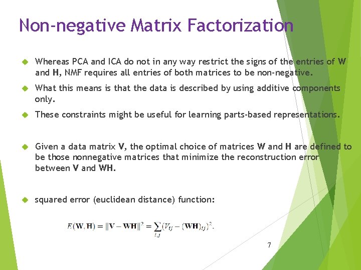
Non-negative Matrix Factorization Whereas PCA and ICA do not in any way restrict the signs of the entries of W and H, NMF requires all entries of both matrices to be non-negative. What this means is that the data is described by using additive components only. These constraints might be useful for learning parts-based representations. Given a data matrix V, the optimal choice of matrices W and H are defined to be those nonnegative matrices that minimize the reconstruction error between V and WH. squared error (euclidean distance) function: 7

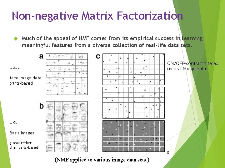
Non-negative Matrix Factorization Much of the appeal of NMF comes from its empirical success in learning meaningful features from a diverse collection of real-life data sets. ON/OFF-contrast filtered natural image data. CBCL face image data parts-based ORL Basis images global rather than parts-based 8 (NMF applied to various image data sets. )

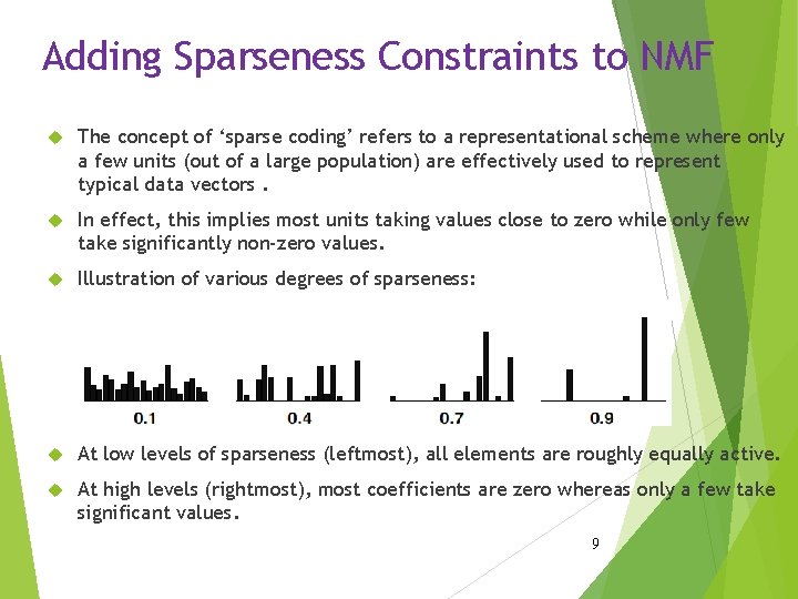
Adding Sparseness Constraints to NMF The concept of ‘sparse coding’ refers to a representational scheme where only a few units (out of a large population) are effectively used to represent typical data vectors. In effect, this implies most units taking values close to zero while only few take significantly non-zero values. Illustration of various degrees of sparseness: At low levels of sparseness (leftmost), all elements are roughly equally active. At high levels (rightmost), most coefficients are zero whereas only a few take significant values. 9

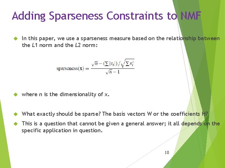
Adding Sparseness Constraints to NMF In this paper, we use a sparseness measure based on the relationship between the L 1 norm and the L 2 norm: where n is the dimensionality of x. What exactly should be sparse? The basis vectors W or the coefficients H? This is a question that cannot be given a general answer; it all depends on the specific application in question. 10

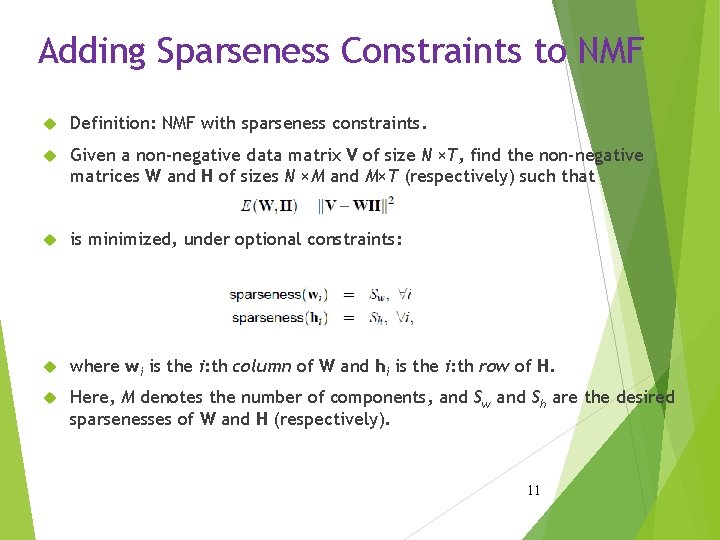
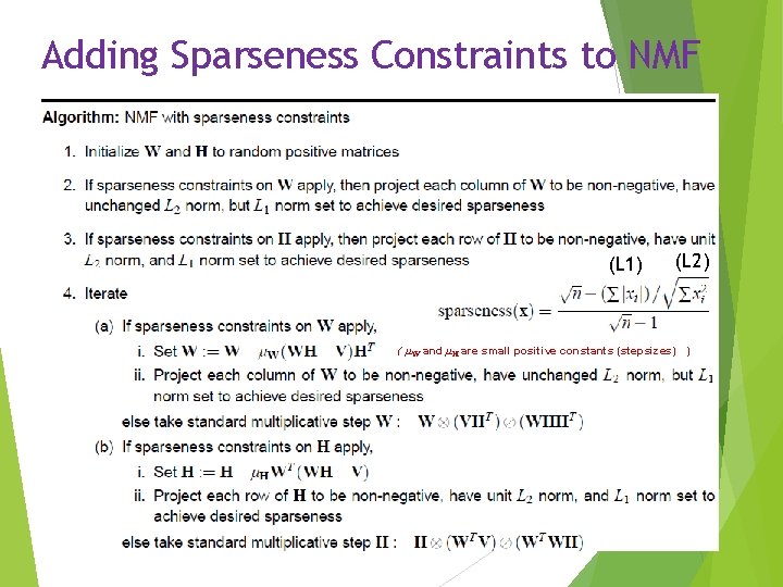
Adding Sparseness Constraints to NMF Definition: NMF with sparseness constraints. Given a non-negative data matrix V of size N ×T, find the non-negative matrices W and H of sizes N ×M and M×T (respectively) such that is minimized, under optional constraints: where wi is the i: th column of W and hi is the i: th row of H. Here, M denotes the number of components, and Sw and Sh are the desired sparsenesses of W and H (respectively). 11

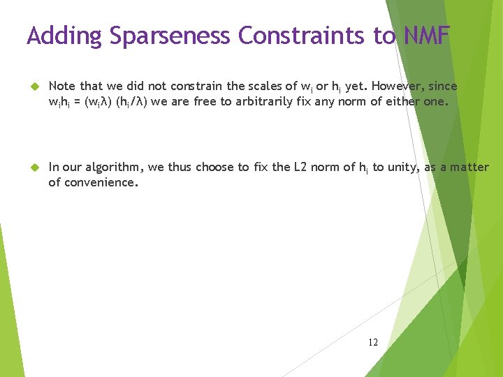
Adding Sparseness Constraints to NMF Note that we did not constrain the scales of wi or hi yet. However, since wihi = (wiλ) (hi/λ) we are free to arbitrarily fix any norm of either one. In our algorithm, we thus choose to fix the L 2 norm of hi to unity, as a matter of convenience. 12

Adding Sparseness Constraints to NMF (L 1) (L 2) ( μW and μH are small positive constants (stepsizes) ) 13

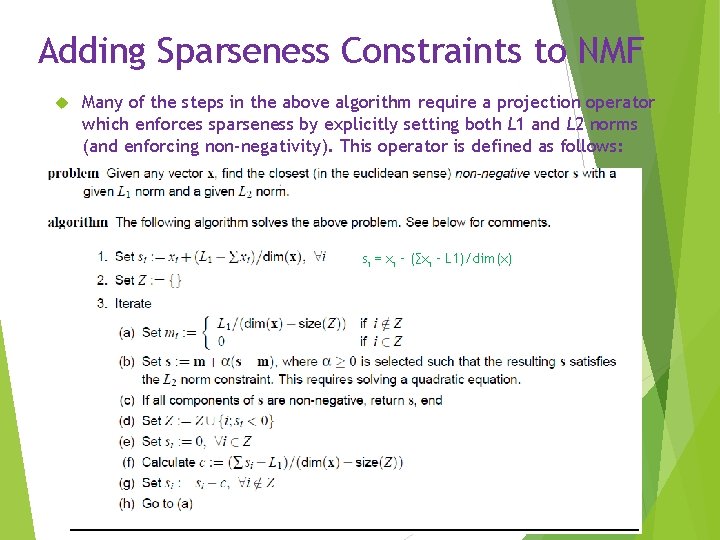
Adding Sparseness Constraints to NMF Many of the steps in the above algorithm require a projection operator which enforces sparseness by explicitly setting both L 1 and L 2 norms (and enforcing non-negativity). This operator is defined as follows: si = xi – (∑xi – L 1)/dim(x) 14

Experiments with Sparseness Constraints In this section, we show that adding sparseness constraints to NMF can make it find parts-based representations in cases where unconstrained NMF does not. In addition, we experimentally verify our claim that the projection operator converges in only a few iterations even when the dimensionality of the vector is high. Representations Learned from Face Image Databases Lee and Seung (1999) originally showed that NMF found a parts-based representation when trained on data from the CBCL database. However, when applied to the ORL data set, in which images are not as well aligned, a global decomposition emerges. 15

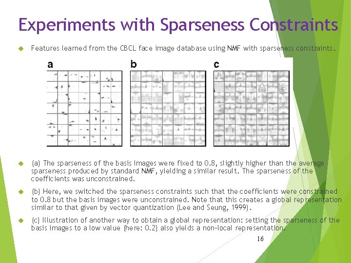
Experiments with Sparseness Constraints Features learned from the CBCL face image database using NMF with sparseness constraints. (a) The sparseness of the basis images were fixed to 0. 8, slightly higher than the average sparseness produced by standard NMF, yielding a similar result. The sparseness of the coefficients was unconstrained. (b) Here, we switched the sparseness constraints such that the coefficients were constrained to 0. 8 but the basis images were unconstrained. Note that this creates a global representation similar to that given by vector quantization (Lee and Seung, 1999). (c) Illustration of another way to obtain a global representation: setting the sparseness of the basis images to a low value (here: 0. 2) also yields a non-local representation. 16

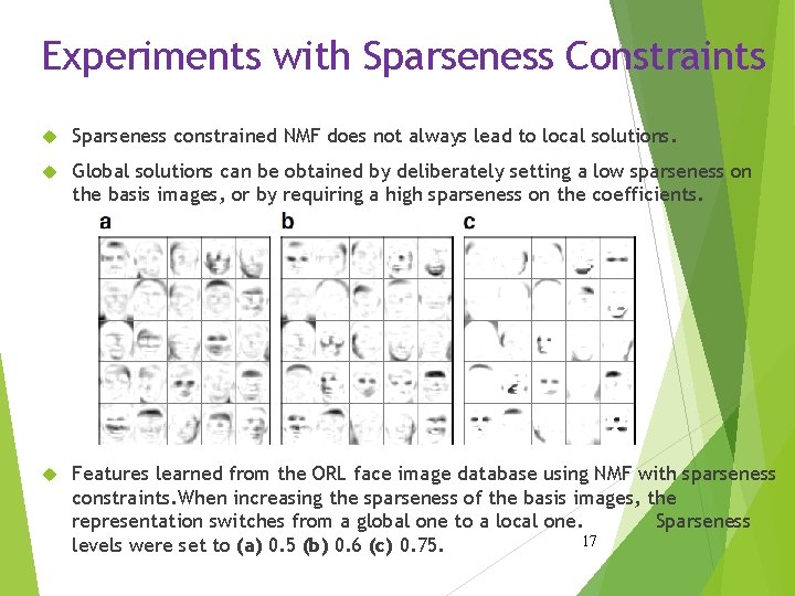
Experiments with Sparseness Constraints Sparseness constrained NMF does not always lead to local solutions. Global solutions can be obtained by deliberately setting a low sparseness on the basis images, or by requiring a high sparseness on the coefficients. Features learned from the ORL face image database using NMF with sparseness constraints. When increasing the sparseness of the basis images, the representation switches from a global one to a local one. Sparseness 17 levels were set to (a) 0. 5 (b) 0. 6 (c) 0. 75.

Experiments with Sparseness Constraints Convergence of Algorithm Implementing the Projection Step To verify the performance of our projection method we performed extensive tests, varying the number of dimensions, the desired degree of sparseness, and the sparseness of the original vector. The desired and the initial degrees of sparseness were set to 0. 1, 0. 3, 0. 5, 0. 7, and 0. 9, and the dimensionality of the problem was set to 2, 3, 5, 10, 50, 100, 500, 1000, 3000, 5000, and 10000. All combinations of sparsenesses and dimensionalities were analyzed. Based on this analysis, the worst case (most iterations on average required) was when the desired degree of sparseness was high (0. 9) but the initial sparseness was low (0. 1). 18

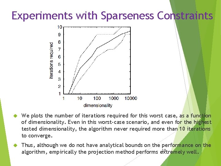
Experiments with Sparseness Constraints We plots the number of iterations required for this worst case, as a function of dimensionality. Even in this worst-case scenario, and even for the highest tested dimensionality, the algorithm never required more than 10 iterations to converge. Thus, although we do not have analytical bounds on the performance on the 19 algorithm, empirically the projection method performs extremely well.

Conclusions Non-negative matrix factorization (NMF) has proven itself a useful tool in the analysis of a diverse range of data. One of its most useful properties is that the resulting decompositions are often intuitive and easy to interpret because they are sparse. Our main contributions of this paper were : (a) to describe a projection operator capable of simultaneously enforcing both L 1 and L 2 norms (b) to show its use in the NMF framework for learning representations that could not be obtained by regular NMF 20