NLTE polarized lines and 3 D structure of

NLTE polarized lines and 3 D structure of magnetic fields P. Mein, N. Mein, M. Faurobert, V. Bommier, J-M. Malherbe, G. Aulanier Magnetic fields cross canopy regions, not easily investigated by extrapolations, between photosphere and chromosphere. Full knowledge of the 3 D structure implies diagnostics extracted from strong NLTE lines. Fortunately, the domain of ‘’weak field ’’ approximation is more extended for such lines (smaller Lande factor, broad lines). The data analysed below are obtained with THEMIS / MSDP and MTR in 589. 6 Na. I (D 1) 610. 27 Ca. I 630. 2 Fe. I (for comparison)

1) D 1 line and facular magnetic flux tubes Problems of filling factor, vertical gradients, MHD models Simulation of line profiles MULTI code with field free assumption, 1 D model Instrumental profile included - Quiet Sun = VAL 3 C model - Circular polarization: I -V profile -Solid line: flux tube, dashed: quiet -Bisector for = +/-8, 16, 24, 32 pm -Weak field assumption B//

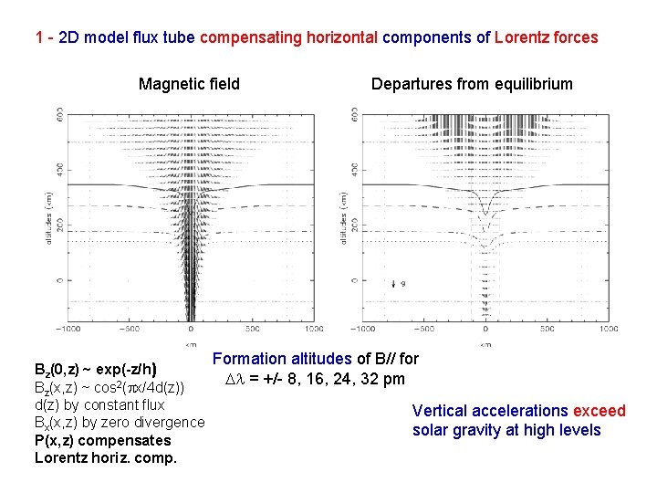
1 - 2 D model flux tube compensating horizontal components of Lorentz forces Magnetic field Bz(0, z) ~ exp(-z/h) Bz(x, z) ~ cos 2( x/4 d(z)) d(z) by constant flux Bx(x, z) by zero divergence P(x, z) compensates Lorentz horiz. comp. Departures from equilibrium Formation altitudes of B// for = +/- 8, 16, 24, 32 pm Vertical accelerations exceed solar gravity at high levels

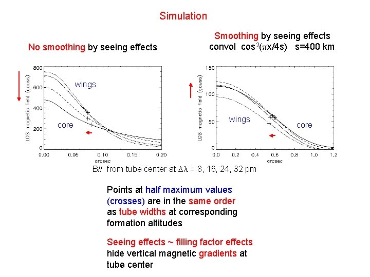
Simulation No smoothing by seeing effects Smoothing by seeing effects convol cos 2( x/4 s) s=400 km wings core wings B// from tube center at = 8, 16, 24, 32 pm Points at half maximum values (crosses) are in the same order as tube widths at corresponding formation altitudes Seeing effects ~ filling factor effects hide vertical magnetic gradients at tube center core

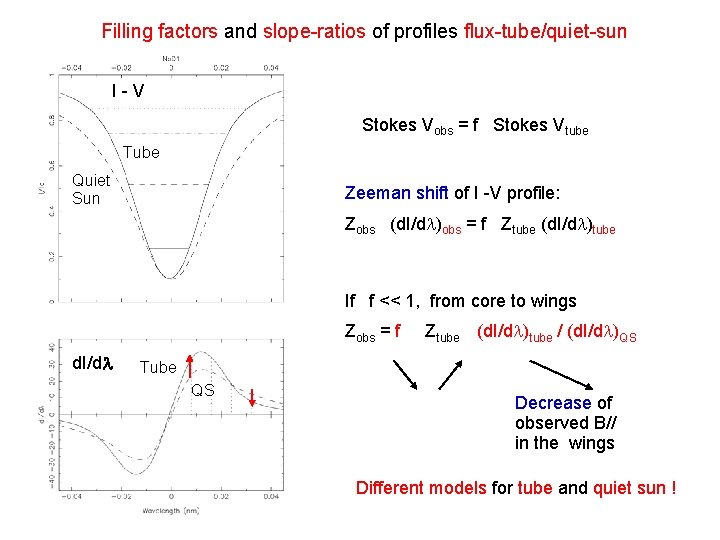
Filling factors and slope-ratios of profiles flux-tube/quiet-sun I-V Stokes Vobs = f Stokes Vtube Tube Quiet Sun Zeeman shift of I -V profile: Zobs (d. I/d )obs = f Ztube (d. I/d )tube If f << 1, from core to wings Zobs = f d. I/d Ztube (d. I/d )tube / (d. I/d )QS Tube QS Decrease of observed B// in the wings Different models for tube and quiet sun !

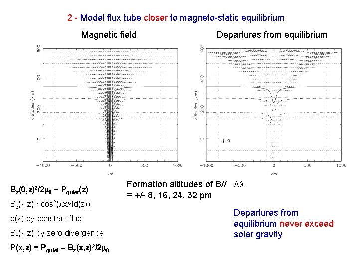
2 - Model flux tube closer to magneto-static equilibrium Magnetic field Bz(0, z)2/2 0 ~ Pquiet(z) Bz(x, z) ~cos 2( x/4 d(z)) d(z) by constant flux Bx(x, z) by zero divergence P(x, z) = Pquiet – Bz(x, z)2/2 0 Departures from equilibrium Formation altitudes of B// = +/- 8, 16, 24, 32 pm Departures from equilibrium never exceed solar gravity

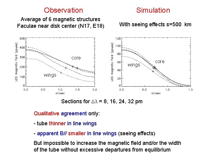
Observation Average of 6 magnetic structures Faculae near disk center (N 17, E 18) Simulation With seeing effects s=500 km core wings Sections for = 8, 16, 24, 32 pm Qualitative agreement only: - tube thinner in line wings - apparent B// smaller in line wings (seeing effects) But impossible to increase the magnetic field and/or the width of the tube without excessive departures from equilibrium

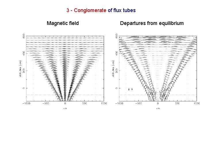
3 - Conglomerate of flux tubes Magnetic field Departures from equilibrium

Observation Simulation Seeing effects s = 700 km Better qualitative agreement (tube width) But magnetic field still too low Coronal magnetic field outside the structure? MHD models, including temperature and velocity fluctuations…? P. Mein, N. Mein, M. Faurobert, G. Aulanier and J-M. Malherbe, A&A 463, 727 (2007)

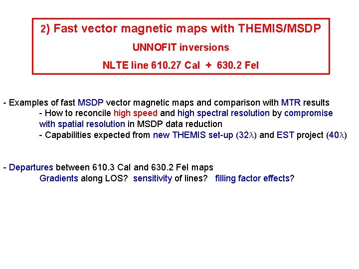
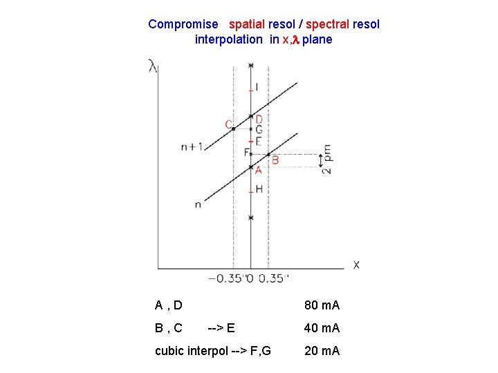
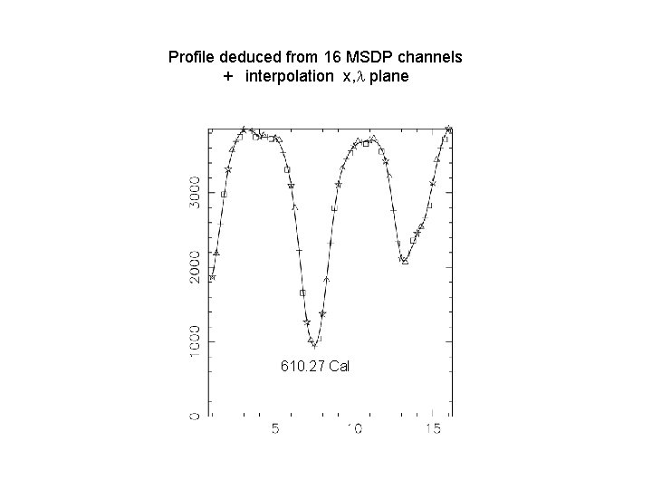
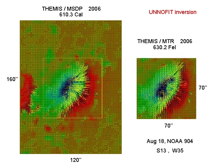
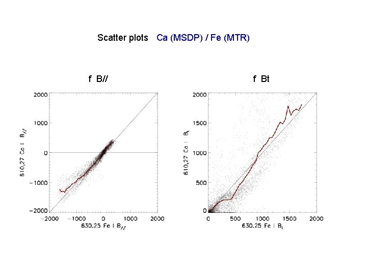
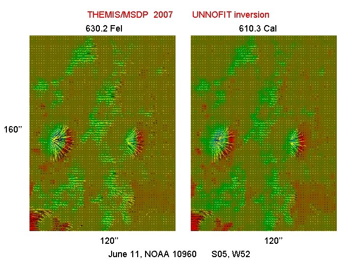
2) Fast vector magnetic maps with THEMIS/MSDP UNNOFIT inversions NLTE line 610. 27 Ca. I + 630. 2 Fe. I - Examples of fast MSDP vector magnetic maps and comparison with MTR results - How to reconcile high speed and high spectral resolution by compromise with spatial resolution in MSDP data reduction - Capabilities expected from new THEMIS set-up (32 ) and EST project (40 ) - Departures between 610. 3 Ca. I and 630. 2 Fe. I maps Gradients along LOS? sensitivity of lines? filling factor effects?

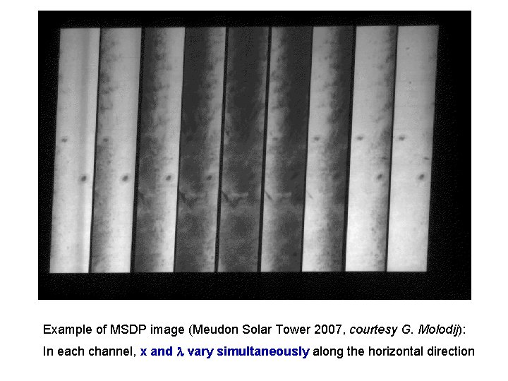
Example of MSDP image (Meudon Solar Tower 2007, courtesy G. Molodij): In each channel, x and vary simultaneously along the horizontal direction

Compromise spatial resol / spectral resol interpolation in x, plane A, D B, C 80 m. A --> E cubic interpol --> F, G 40 m. A 20 m. A

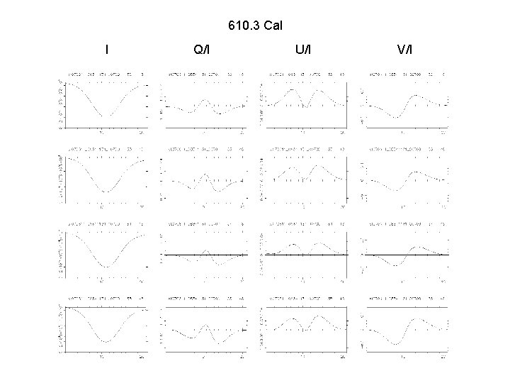
Profile deduced from 16 MSDP channels + interpolation x, plane 610. 27 Ca. I

THEMIS / MSDP 610. 3 Ca. I 2006 UNNOFIT inversion THEMIS / MTR 2006 630. 2 Fe. I 160’’ 70’’ Aug 18, NOAA 904 S 13 , W 35 120’’

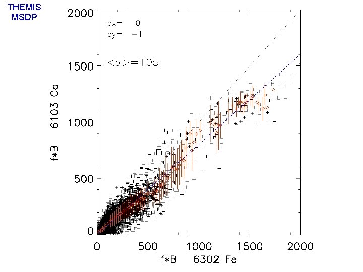
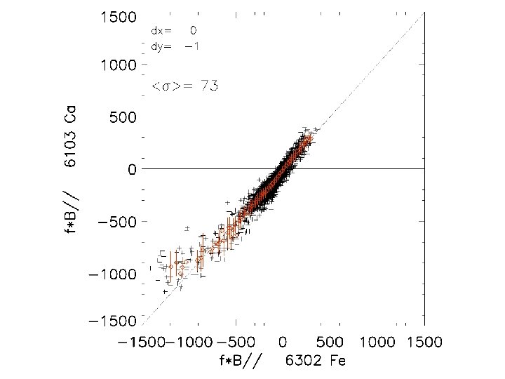
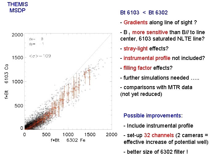
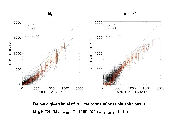
Scatter plots Ca (MSDP) / Fe (MTR) f B// f Bt

THEMIS/MSDP 2007 UNNOFIT inversion 630. 2 Fe. I 610. 3 Ca. I 160’’ 120’’ June 11, NOAA 10960 120’’ S 05, W 52

610. 3 Ca. I I Q/I U/I V/I

THEMIS MSDP

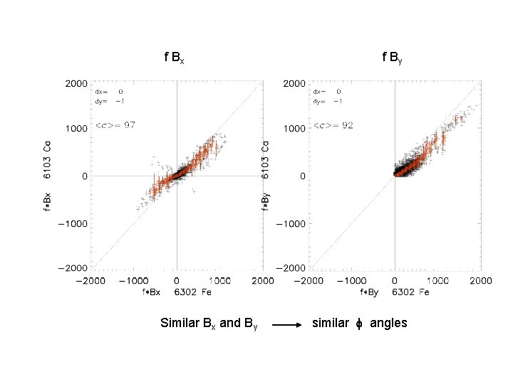
f Bx Similar Bx and By f By similar f angles

THEMIS MSDP Bt 6103 < Bt 6302 - Gradients along line of sight ? - B t more sensitive than B// to line center, 6103 saturated NLTE line? - stray-light effects? - instrumental profile not included? - filling factor effects? - further simulations needed …. . - comparisons with MTR data (not yet reduced) Possible improvements: - Include instrumental profile - set-up 32 channels (2 cameras = effective increase of potential well) - better size of 6302 filter !

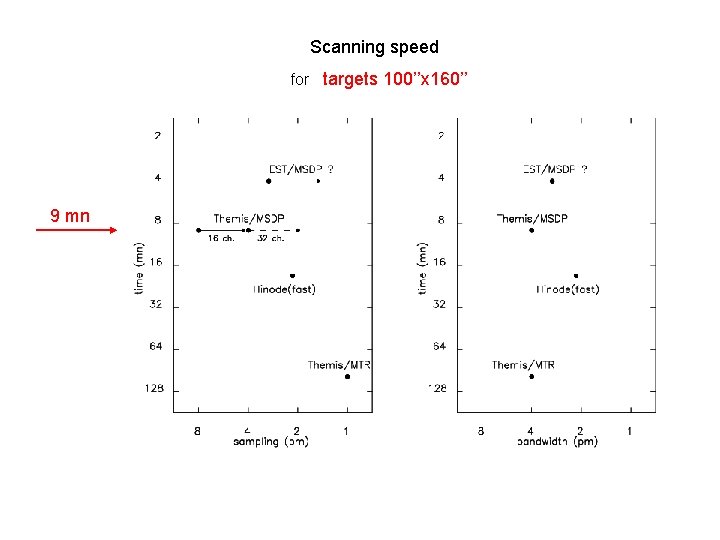
Scanning speed for targets 100’’x 160’’ 9 mn

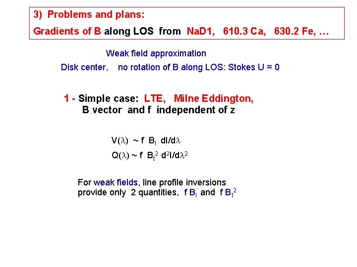
3) Problems and plans: Gradients of B along LOS from Na. D 1, 610. 3 Ca, 630. 2 Fe, … Weak field approximation Disk center, no rotation of B along LOS: Stokes U = 0 1 - Simple case: LTE, Milne Eddington, B vector and f independent of z V( ) ~ f Bl d. I/d Q( ) ~ f Bt 2 d 2 I/d 2 For weak fields, line profile inversions provide only 2 quantities, f Bl and f Bt 2

Bt * f 1/2 Below a given level of c 2 the range of possible solutions is larger for (Btransverse * f ) than for (Btransverse * f ½) ?

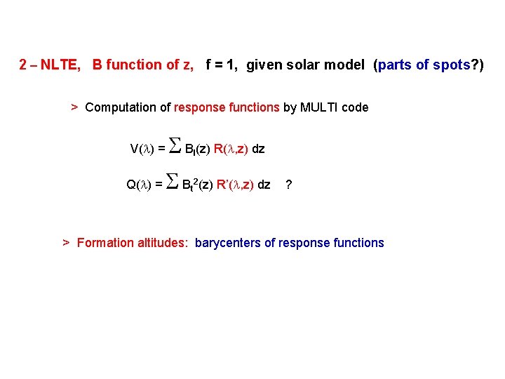
2 – NLTE, B function of z, f = 1, given solar model (parts of spots? ) > Computation of response functions by MULTI code V( ) = Q( ) = S B (z) R( , z) dz l SB t 2(z) R’( , z) dz ? > Formation altitudes: barycenters of response functions

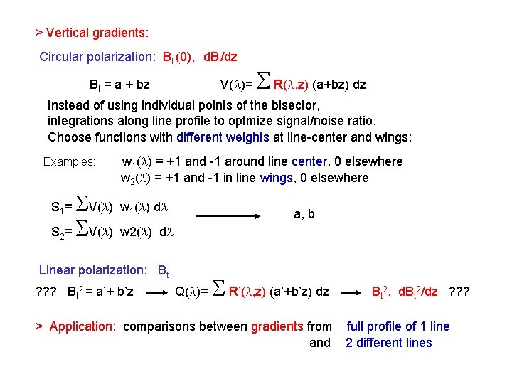
> Vertical gradients: Circular polarization: Bl (0), d. Bl/dz Bl = a + bz V( )= S R( , z) (a+bz) dz Instead of using individual points of the bisector, integrations along line profile to optmize signal/noise ratio. Choose functions with different weights at line-center and wings: Examples: SV( ) S = SV( ) w 1( ) = +1 and -1 around line center, 0 elsewhere w 2( ) = +1 and -1 in line wings, 0 elsewhere S 1= w 1( ) d 2 w 2( ) d a, b Linear polarization: Bt ? ? ? Bt 2 = a’+ b’z Q( )= S R’( , z) (a’+b’z) dz Bt 2, d. Bt 2/dz ? ? ? > Application: comparisons between gradients from full profile of 1 line and 2 different lines

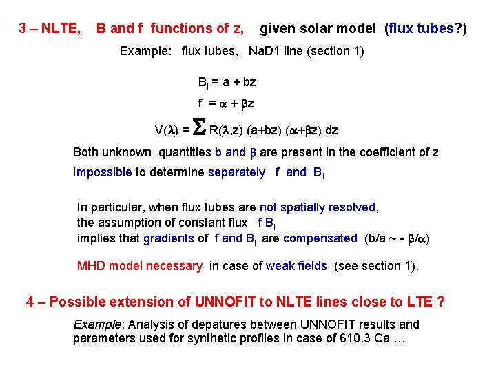
3 – NLTE, B and f functions of z, given solar model (flux tubes? ) Example: flux tubes, Na. D 1 line (section 1) Bl = a + bz f = a + bz V( ) = S R( , z) (a+bz) dz Both unknown quantities b and b are present in the coefficient of z Impossible to determine separately f and Bl In particular, when flux tubes are not spatially resolved, the assumption of constant flux f Bl implies that gradients of f and Bl are compensated (b/a ~ - b/a) MHD model necessary in case of weak fields (see section 1). 4 – Possible extension of UNNOFIT to NLTE lines close to LTE ? Example: Analysis of depatures between UNNOFIT results and parameters used for synthetic profiles in case of 610. 3 Ca …