MS 101 Algorithms Instructor Neelima Gupta nguptacs du

MS 101: Algorithms Instructor Neelima Gupta ngupta@cs. du. ac. in

Table of Contents Greedy Algorithms

What is greedy approach? �Choosing a current best solution without worrying about future. In other words the choice does not depend upon future sub-problems. �Such algorithms are locally optimal, �For some problems, as we will see shortly, this local optimal is global optimal also and we are happy.

General ‘Greedy’ Approach �Step 1: �Choose the current best solution. �Step 2: �Obtain greedy solution on the rest.

When to use? �There must be a greedy choice to make. �The problem must have an optimal substructure.

Activity Selection Problem �Given a set of activities, S = {a 1, a 2, …, an} that need to use some resource. �Each activity ai has a possible start time si & finish time fi, such that 0 si < fi < �We need to allocate the resource in a compatible manner, such that the number of activities getting the resource is maximized. �The resource can be used by one and only one activity at any given time. .

Activity Selection Problem �Two activities ai and aj are said to be compatible, if the interval they span do not overlap. . . i. e. fi sj or fj si �Example: �Consider activities: a 1, a 2, a 3, a 4 s 1 ----f 1 s 2 -----f 2 s 3 ------f 3 s 4 ------f 4 �Here a 1 is compatible with a 3 & a 4 �a 2 is compatible with a 3 & a 4 �But a 3 and a 4 themselves are not compatible.

Activity Selection Problem �Solution: Applying the general greedy algorithm �Select the current best choice, a 1 add it to the solution set. �Construct a subset S’ of all activities compatible with a 1, find the optimal solution of this subset. �Join the two.

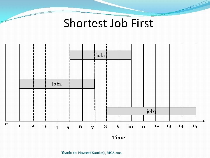
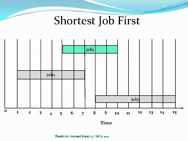
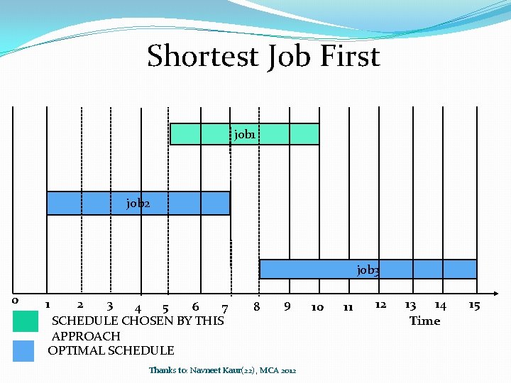
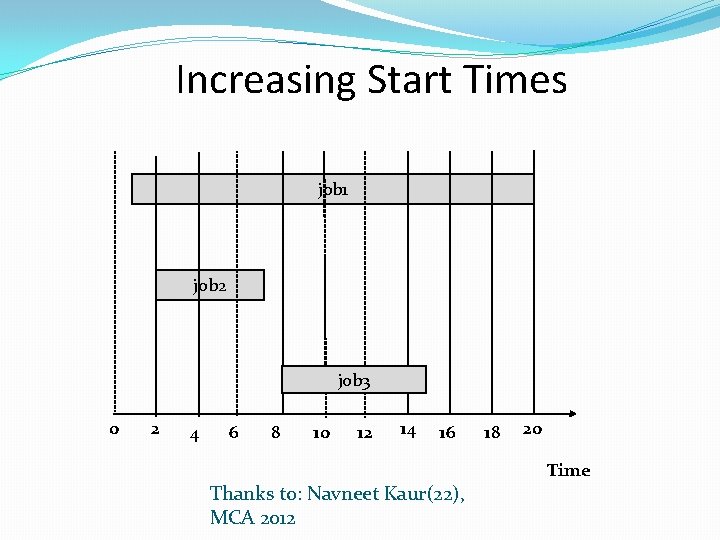
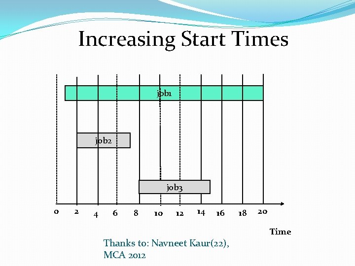
Lets think of some possible greedy solutions �Shortest Job First �In the order of increasing start times �In the order of increasing finish times

Shortest Job First job 1 job 2 job 3 0 1 2 3 4 5 6 7 8 9 Time Thanks to: Navneet Kaur(22), MCA 2012 10 11 12 13 14 15

Shortest Job First job 1 job 2 job 3 0 1 2 3 4 5 6 7 8 9 Time Thanks to: Navneet Kaur(22), MCA 2012 10 11 12 13 14 15

Shortest Job First job 1 job 2 job 3 0 1 2 3 4 5 6 7 SCHEDULE CHOSEN BY THIS APPROACH OPTIMAL SCHEDULE 8 9 Thanks to: Navneet Kaur(22), MCA 2012 10 11 12 13 14 Time 15

Increasing Start Times job 1 job 2 job 3 0 2 4 6 8 10 12 14 16 Thanks to: Navneet Kaur(22), MCA 2012 18 20 Time

Increasing Start Times job 1 job 2 job 3 0 2 4 6 8 10 12 14 16 Thanks to: Navneet Kaur(22), MCA 2012 18 20 Time

Increasing Start Times job 1 job 2 job 3 0 2 14 4 6 8 10 12 SCHEDULE CHOSEN BY THIS APPROACH OPTIMAL SCHEDULE 16 Thanks to: Navneet Kaur(22), MCA 2012 18 20 Time

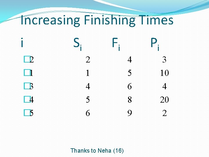
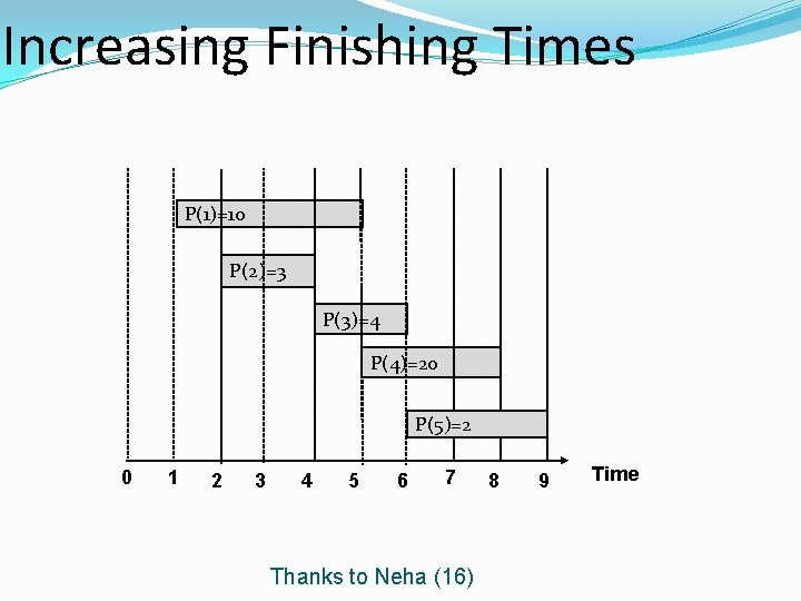
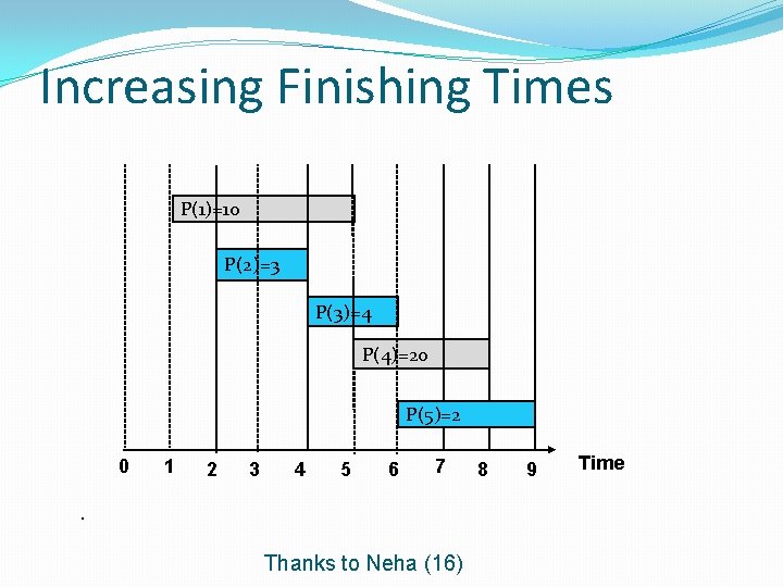
Increasing Finishing Times i � 2 � 1 � 3 � 4 � 5 Si Fi 2 1 4 5 6 Thanks to Neha (16) Pi 4 5 6 8 9 3 10 4 20 2

Increasing Finishing Times P(1)=10 P(2)=3 P(3)=4 P(4)=20 P(5)=2 0 1 2 3 4 5 6 7 Thanks to Neha (16) 8 9 Time

Increasing Finishing Times P(1)=10 P(2)=3 P(3)=4 P(4)=20 P(5)=2 0 1 2 3 4 5 6 7 . Thanks to Neha (16) 8 9 Time

ACTIVITY SELECTION PROBLEM We include a₁ in the solution. And then recurse on S′ = {aₓ ԑ S-{a₁} : aₓ is compatible with a₁} where S is input set of activities. Thanks to: Navneet Kaur(22), MCA 2012

Proving the Optimality

Scheduling Jobs with Processing times and Deadlines �Jobs are given with processing times pi and deadlines d i. �There is no specified start time. A job can be scheduled at any time. Algorithm decides the start time ( and hence the finish time) of a job. �Let fi be the time at which a job finishes as per some schedule. Then its lateness is defined as li = fi – di if fi>di 0 , otherwise �Aim : minimize max lateness i. e. minimize max{li}

Figures from Anjali, Hemant

Possible Greedy Approaches �Shortest Job First: completely ignores half of the input data viz. the deadlines �Doesn’t work : � t 1 = 1, d 1=100, t 2=10, d 2=10 �Minimum Slackness First �Doesn’t work : � t 1 = 1, d 1=2, t 2=10, d 2=10 �Earliest Deadline First: completely ignores the other half of the input data viz. the processing time…. but it works…. gives the optimal

SJF fails: figure from Anjali, Hemant back

q. Minimum Slackness First � Let si be the time by which the job must be assigned to meet the deadline. i. e. si = di – pi �Let the last job scheduled finishes at time t. Then slacktime for job i is defined as sti = si – t. �Thus slack time represents, how much we can wait/defer to schedule the ith job. �We should schedule the next job for which this time is minimum. i. e. sti is minimum. Since t is same for all the jobs, the job with minimum si is scheduled next.

MSF fails: figure from Anjali, Hemant back

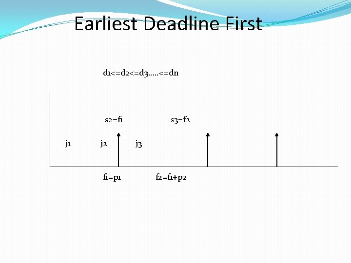
Earliest Deadline First d 1<=d 2<=d 3…. . <=dn s 2=f 1 j 2 f 1=p 1 s 3=f 2 j 3 f 2=f 1+p 2

Exchange Argument • Let O be an optimal solution and S be the solution obtained by our greedy. • Gradually we transform O into S without hurting its (O’s) quality. Thereby implying that |O| = |S|. • Hence proving that greedy is optimal.

q. Inversion We say that a schedule A has an inversion if a job i with deadline di is scheduled before another job j with earlier deadline( dj<di). q Idle Time -The time that passes during a gap -There is work to be done, yet for some reason the machine is sitting idle.

Earliest Deadline First �Claim: Our schedule has no inversions and no idle time…. trivial �Clearly Optimal has no idle time. � 1. All schedules with no inversion and no idle time has same maximum lateness �Proof: � 2. There is an optimal schedule with no inversion and no idle time. �A. If O (an optimal) has an inversion there is a pair of jobs I an j such that j is scheduled immediately after I and d_j < d_i…. i. e. pair of inverted jobs that are consecutive. �Proof: �B. The new swapped schedule has maximum lateness no larger than that of O. �Proof:

Proof of 1. : Anjali, Hemant

Network Design Problems �Given a set of routers placed at n locations V = {v 1 … vn} �We want to connect them in a cheapest way. �Claim: The minimum cost solution to the above problem is a tree.

Minimum Spanning Tree �Assume that all edges have distinct edge costs. We’ll remove this restriction later. �Greedy Approaches: �Kruskal �Prim’s �Reverse Delete �Cut Property: Let S be a non-trivial subset of V, let e = (v, w) be the minimum weight edge with one end in S and the other end in V – S. Then every MST contains e.