MS 101 Algorithms Instructor Neelima Gupta nguptacs du











- Slides: 92

MS 101: Algorithms Instructor Neelima Gupta ngupta@cs. du. ac. in

Table Of Contents Introduction to some tools to designing algorithms through Sorting • Iterative • Divide and Conquer

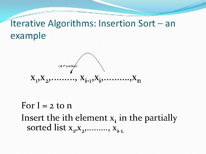
Iterative Algorithms: Insertion Sort – an example (at rth position) x 1, x 2, . . , xi-1, xi, . . . . …, xn For I = 2 to n Insert the ith element xi in the partially sorted list x 1, x 2, . . , xi-1.

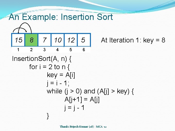
An Example: Insertion Sort 15 8 7 1 2 3 10 12 5 4 5 At Iteration 1: key = 8 6 Insertion. Sort(A, n) { for i = 2 to n { key = A[i] j = i - 1; while (j > 0) and (A[j] > key) { A[j+1] = A[j] j=j-1 } Thanks Brijesh Kumar (08) : MCA -12

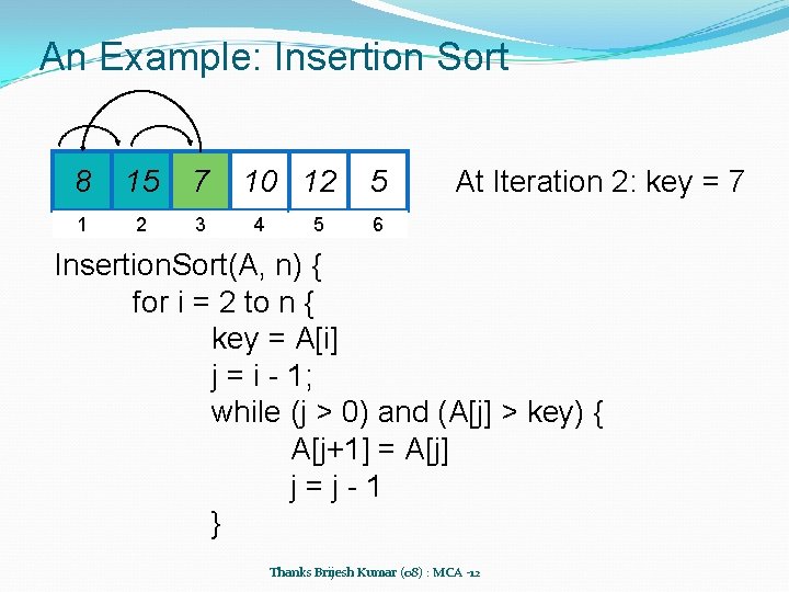
An Example: Insertion Sort 8 15 7 1 2 3 10 12 4 5 5 At Iteration 2: key = 7 6 Insertion. Sort(A, n) { for i = 2 to n { key = A[i] j = i - 1; while (j > 0) and (A[j] > key) { A[j+1] = A[j] j=j-1 } Thanks Brijesh Kumar (08) : MCA -12

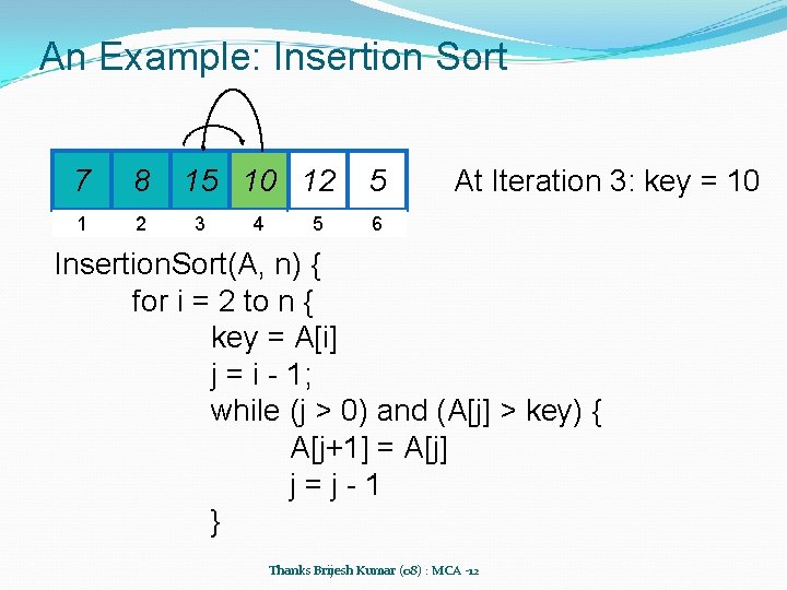
An Example: Insertion Sort 7 8 1 2 15 10 12 3 4 5 5 At Iteration 3: key = 10 6 Insertion. Sort(A, n) { for i = 2 to n { key = A[i] j = i - 1; while (j > 0) and (A[j] > key) { A[j+1] = A[j] j=j-1 } Thanks Brijesh Kumar (08) : MCA -12

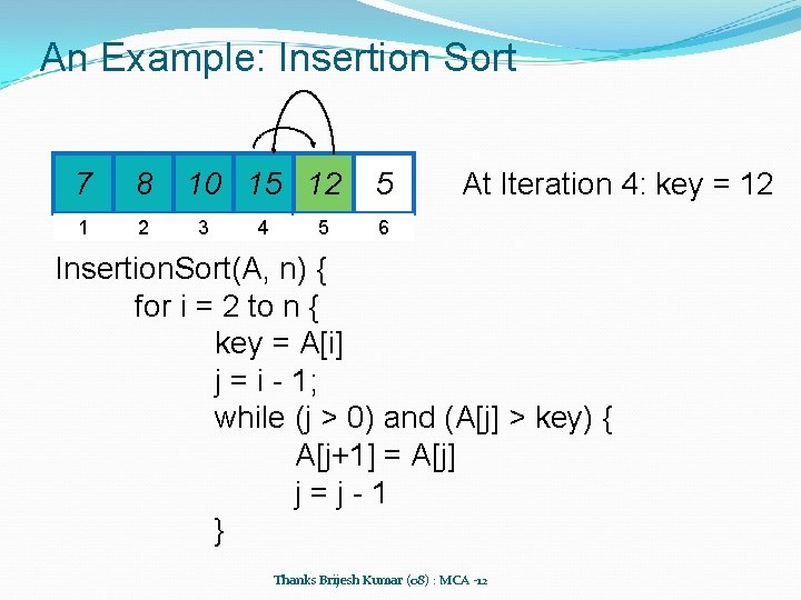
An Example: Insertion Sort 7 8 1 2 10 15 12 3 4 5 5 At Iteration 4: key = 12 6 Insertion. Sort(A, n) { for i = 2 to n { key = A[i] j = i - 1; while (j > 0) and (A[j] > key) { A[j+1] = A[j] j=j-1 } Thanks Brijesh Kumar (08) : MCA -12

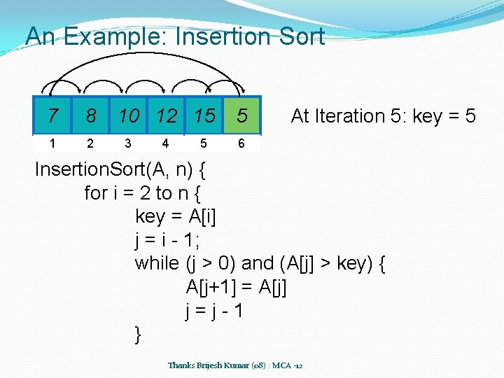
An Example: Insertion Sort 7 8 1 2 10 12 15 3 4 5 5 At Iteration 5: key = 5 6 Insertion. Sort(A, n) { for i = 2 to n { key = A[i] j = i - 1; while (j > 0) and (A[j] > key) { A[j+1] = A[j] j=j-1 } Thanks Brijesh Kumar (08) : MCA -12

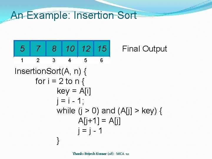
An Example: Insertion Sort 5 7 8 1 2 3 10 12 15 4 5 Final Output 6 Insertion. Sort(A, n) { for i = 2 to n { key = A[i] j = i - 1; while (j > 0) and (A[j] > key) { A[j+1] = A[j] j=j-1 } Thanks Brijesh Kumar (08) : MCA -12

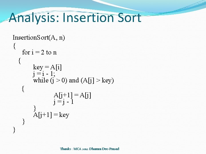
Analysis: Insertion Sort Insertion. Sort(A, n) { for i = 2 to n { key = A[i] j = i - 1; while (j > 0) and (A[j] > key) { A[j+1] = A[j] j=j-1 } A[j+1] = key } } Thanks : MCA 2012 Dharam Deo Prasad

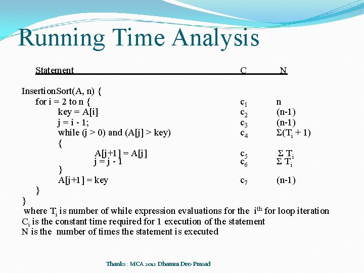
Running Time Analysis Statement C N Insertion. Sort(A, n) { for i = 2 to n { c 1 n key = A[i] c 2 (n-1) j = i - 1; c 3 (n-1) while (j > 0) and (A[j] > key) c 4 Σ(Ti + 1) { A[j+1] = A[j] c 5 Σ Ti j=j-1 c 6 Σ Ti } A[j+1] = key c 7 (n-1) } } where Ti is number of while expression evaluations for the ith for loop iteration Ci is the constant time required for 1 execution of the statement N is the number of times the statement is executed Thanks : MCA 2012 Dharam Deo Prasad

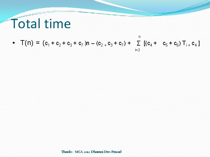
Total time n • T(n) = (c 1 + c 2 + c 3 + c 7 )n – (c 2 + c 3 + c 7) + ∑ [(c 4 + i=2 Thanks : MCA 2012 Dharam Deo Prasad c 5 + c 6) Ti + c 4 ]

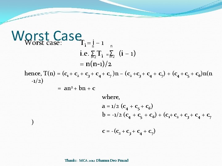
Worst Case. T = i – 1 Worst case: i n n ∑ (i – 1) ∑ i = i. e. T i=2 = n(n-1)/2 hence, T(n) = (c 1 + c 2 + c 3 + c 4 + c 7 )n – (c 2 +c 3 + c 4 + c 7) + (c 4 + c 5 + c 6)n(n -1/2) = an 2 + bn + c where, a = 1/2 (c 4 + c 5 + c 6) b = -1/2 (c 4 + c 5 + c 6) + (c 1+ c 2 + c 3 + c 4 + c 7 ) c = -(c 2 + c 3 + c 4 + c 7) Thanks : MCA 2012 Dharam Deo Prasad

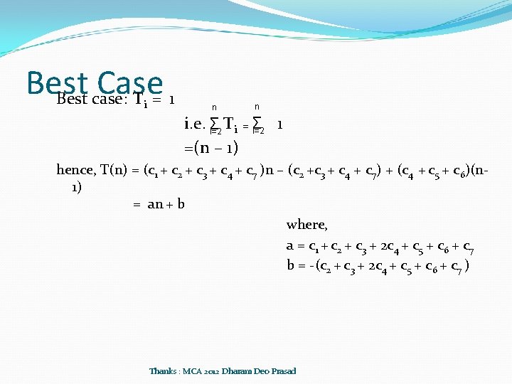
Best Case Best case: T = 1 i n n ∑ 1 ∑ i = i. e. T i=2 =(n – 1) hence, T(n) = (c 1 + c 2 + c 3 + c 4 + c 7 )n – (c 2 +c 3 + c 4 + c 7) + (c 4 + c 5 + c 6)(n 1) = an + b where, a = c 1 + c 2 + c 3 + 2 c 4 + c 5 + c 6 + c 7 b = -(c 2 + c 3 + 2 c 4 + c 5 + c 6 + c 7 ) Thanks : MCA 2012 Dharam Deo Prasad

Analysis of Algorithms �Before we move ahead, let us define the notion of analysis of algorithms more formally

Input Size �Time and space complexity �This is generally a function of the input size �How we characterize input size depends: � Sorting: number of input items � Multiplication: total number of bits � Graph algorithms: number of nodes & edges � Etc

Lower Bounds �Please understand the following statements carefully. �Any algorithm that sorts by removing at most one inversion per comparison does at least n(n-1)/2 comparisons in the worst case. �Hence Insertion Sort is optimal in this category of algorithms.

Optimal? �What do you mean by the term “Optimal”? �Answer: If an algorithm runs as fast in the worst case as it is possible (in the best case), we say that the algorithm is optimal. i. e if the worst case performance of an algorithm matches the lower bound, the algorithm is said to be “optimal”

Inversion : - Example : 4, 2, 3 No. of pairs = 3 C 2 , out of which �(4, 2) is out of order i. e. inversion �(2, 3) is in order �(4, 3) inversion Thanks to: Dileep Jaiswal (11) : MCA 2012

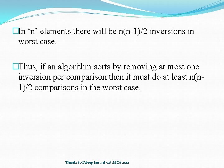
�In ‘n’ elements there will be n(n-1)/2 inversions in worst case. �Thus, if an algorithm sorts by removing at most one inversion per comparison then it must do at least n(n 1)/2 comparisons in the worst case. Thanks to: Dileep Jaiswal (11) : MCA 2012

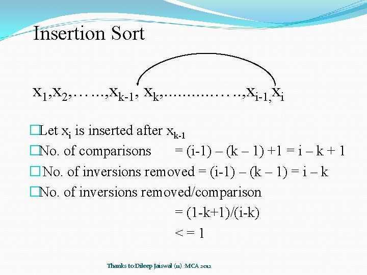
Insertion Sort x 1, x 2, …. . . , xk-1, xk, . . . …. . , xi-1, xi �Let xi is inserted after xk-1 �No. of comparisons = (i-1) – (k – 1) +1 = i – k + 1 � No. of inversions removed = (i-1) – (k – 1) = i – k �No. of inversions removed/comparison = (1 -k+1)/(i-k) <=1 Thanks to: Dileep Jaiswal (11) : MCA 2012

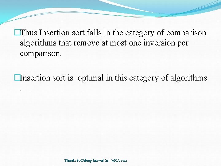
�Thus Insertion sort falls in the category of comparison algorithms that remove at most one inversion per comparison. �Insertion sort is optimal in this category of algorithms. Thanks to: Dileep Jaiswal (11) : MCA 2012

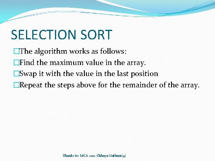
SELECTION SORT �The algorithm works as follows: �Find the maximum value in the array. �Swap it with the value in the last position �Repeat the steps above for the remainder of the array. Thanks to: MCA 2012 Chhaya Nathani(9)

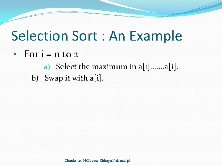
Selection Sort : An Example § For i = n to 2 a) Select the maximum in a[1]. . . . a[i]. b) Swap it with a[i]. Thanks to: MCA 2012 Chhaya Nathani(9)

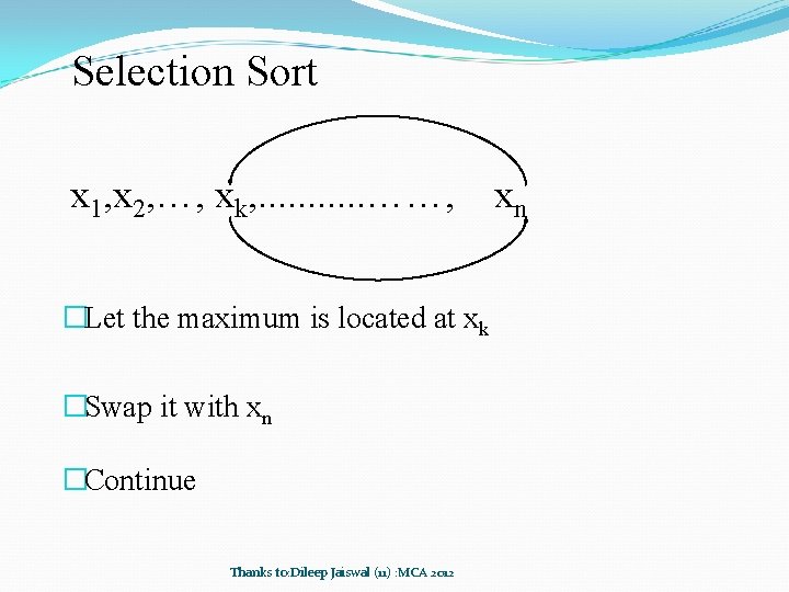
Selection Sort x 1, x 2, …, xk, . . . ……, �Let the maximum is located at xk �Swap it with xn �Continue Thanks to: Dileep Jaiswal (11) : MCA 2012 xn

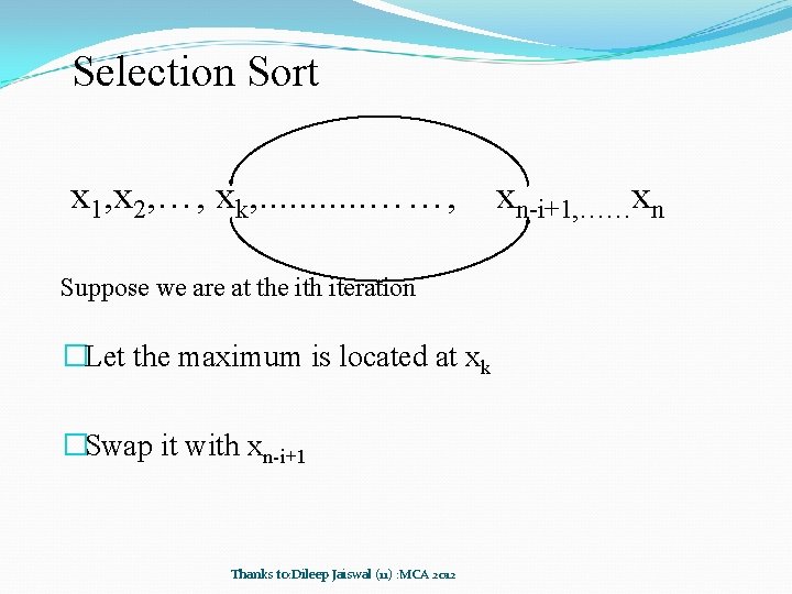
Selection Sort x 1, x 2, …, xk, . . . ……, Suppose we are at the ith iteration �Let the maximum is located at xk �Swap it with xn-i+1 Thanks to: Dileep Jaiswal (11) : MCA 2012 xn-i+1, ……xn

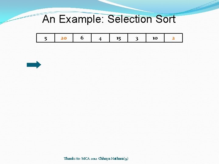
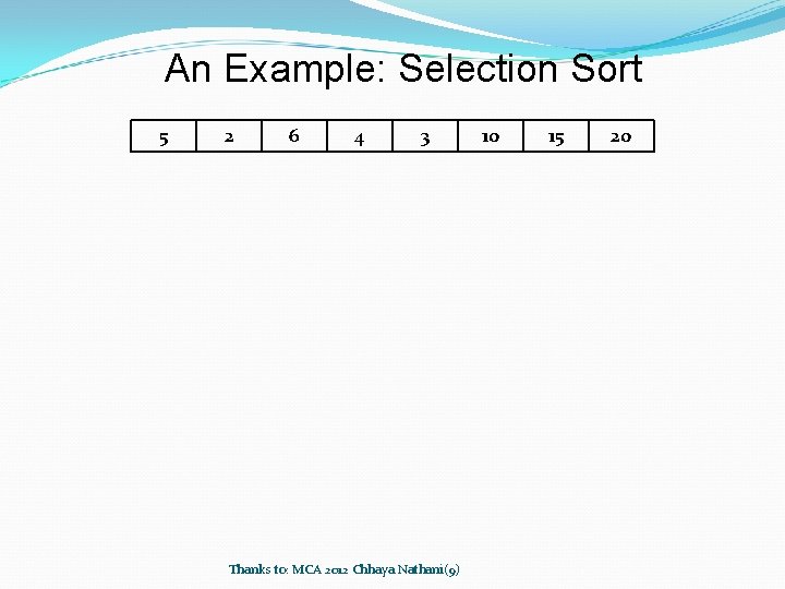
An Example: Selection Sort 5 20 6 4 15 Thanks to: MCA 2012 Chhaya Nathani(9) 3 10 2

An Example: Selection Sort 5 2 6 4 15 Thanks to: MCA 2012 Chhaya Nathani(9) 3 10 20

An Example: Selection Sort 5 2 6 4 10 Thanks to: MCA 2012 Chhaya Nathani(9) 3 15 20

An Example: Selection Sort 5 2 6 4 3 Thanks to: MCA 2012 Chhaya Nathani(9) 10 15 20

An Example: Selection Sort 5 2 3 4 6 10 Thanks to: MCA 2012 Chhaya Nathani(9) 15 20

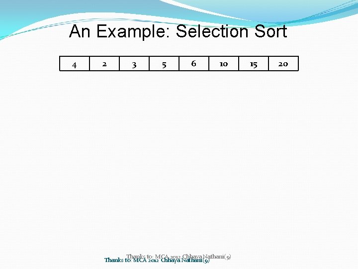
An Example: Selection Sort 4 2 3 5 6 10 Thanks to: MCA 2012 Chhaya Nathani(9) 15 20

An Example: Selection Sort 3 2 4 5 6 10 Thanks to: MCA 2012 Chhaya Nathani(9) 15 20

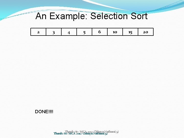
An Example: Selection Sort 2 3 4 5 6 10 DONE!!!! Thanks to: MCA 2012 Chhaya Nathani(9) 15 20

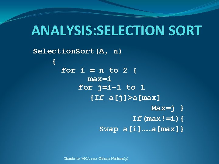
ANALYSIS: SELECTION SORT Selection. Sort(A, n) { for i = n to 2 { max=i for j=i-1 to 1 {If a[j]>a[max] Max=j } If(max!=i){ Swap a[i]……a[max]} Thanks to: MCA 2012 Chhaya Nathani(9)

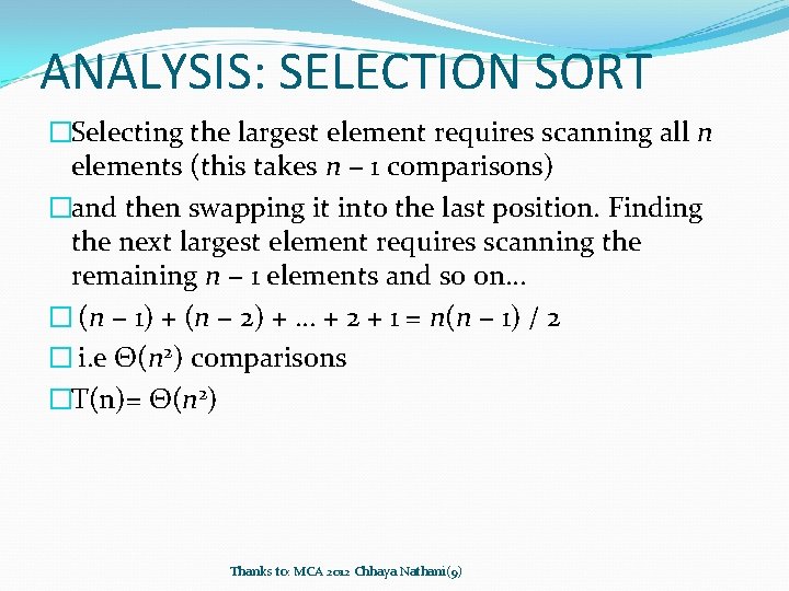
ANALYSIS: SELECTION SORT �Selecting the largest element requires scanning all n elements (this takes n − 1 comparisons) �and then swapping it into the last position. Finding the next largest element requires scanning the remaining n − 1 elements and so on. . . � (n − 1) + (n − 2) +. . . + 2 + 1 = n(n − 1) / 2 � i. e Θ(n 2) comparisons �T(n)= Θ(n 2) Thanks to: MCA 2012 Chhaya Nathani(9)

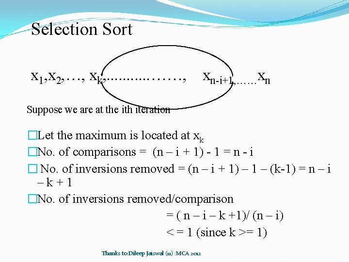
Selection Sort x 1, x 2, …, xk, . . . ……, xn-i+1, ……xn Suppose we are at the ith iteration �Let the maximum is located at xk �No. of comparisons = (n – i + 1) - 1 = n - i � No. of inversions removed = (n – i + 1) – 1 – (k-1) = n – i –k+1 �No. of inversions removed/comparison = ( n – i – k +1)/ (n – i) < = 1 (since k >= 1) Thanks to: Dileep Jaiswal (11) : MCA 2012

�Thus Selection sort also falls in category of comparison algorithms that remove at most one inversion per comparison. �Selection sort is also optimal in this category of algorithms. Thanks to: Dileep Jaiswal (11) : MCA 2012

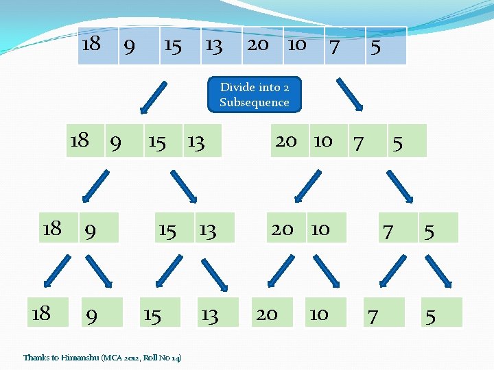
Merge Sort (Divide and Conquer Technique) § Divide the list into nearly equal halves § Sort each half recursively § Merge these lists Thanks to: Gaurav Gulzar (MCA -11)

18 9 15 13 20 10 7 5 Divide into 2 Subsequence 18 9 15 13 15 15 Thanks to Himanshu (MCA 2012, Roll No 14) 13 13 20 10 7 5 20 10 7 7 5 5

Next Sort the 2 subsequences and merge them. Thanks to Himanshu (MCA 2012, Roll No 14)

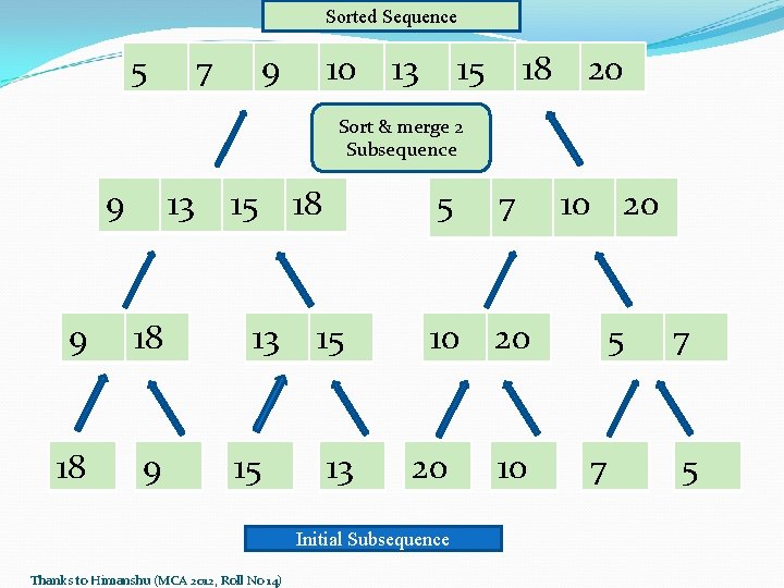
Sorted Sequence 5 7 9 10 13 15 18 20 Sort & merge 2 Subsequence 9 13 9 18 18 9 15 18 13 15 5 15 13 10 20 20 Initial Subsequence Thanks to Himanshu (MCA 2012, Roll No 14) 7 10 5 7 7 5

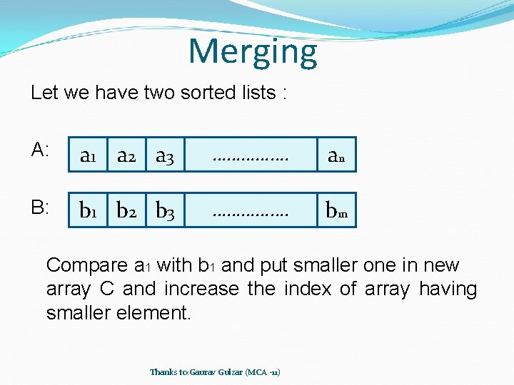
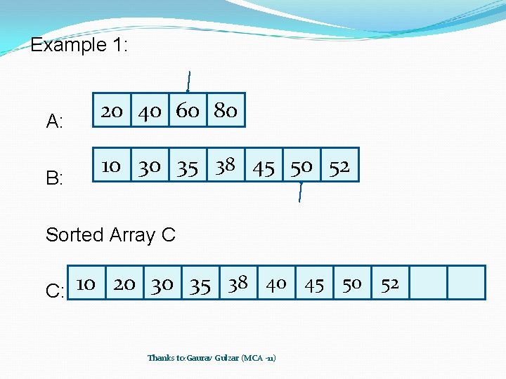
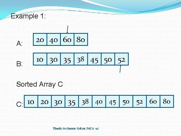
Merging Let we have two sorted lists : A: a 1 a 2 a 3 ……………. an B: b 1 b 2 b 3 ……………. bm Compare a 1 with b 1 and put smaller one in new array C and increase the index of array having smaller element. Thanks to: Gaurav Gulzar (MCA -11)

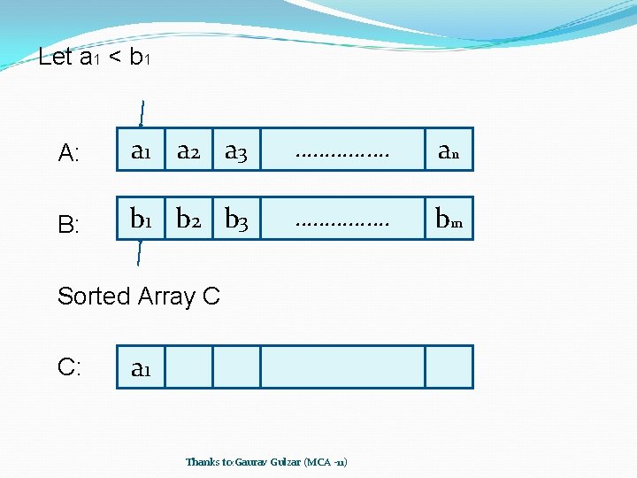
Let a 1 < b 1 A: a 1 a 2 a 3 ……………. an B: b 1 b 2 b 3 ……………. bm Sorted Array C C: a 1 Thanks to: Gaurav Gulzar (MCA -11)

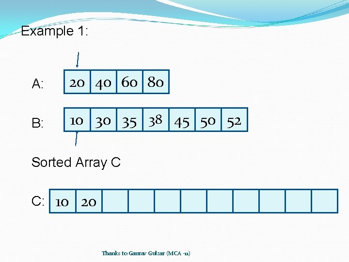
Example 1: A: 20 40 60 80 B: 10 30 35 38 45 50 52 Sorted Array C C: 10 20 Thanks to: Gaurav Gulzar (MCA -11)

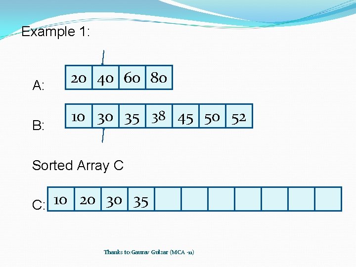
Example 1: A: B: 20 40 60 80 10 30 35 38 45 50 52 Sorted Array C C: 10 20 30 35 Thanks to: Gaurav Gulzar (MCA -11)

Example 1: A: B: 20 40 60 80 10 30 35 38 45 50 52 Sorted Array C 38 10 20 30 35 C: Thanks to: Gaurav Gulzar (MCA -11)

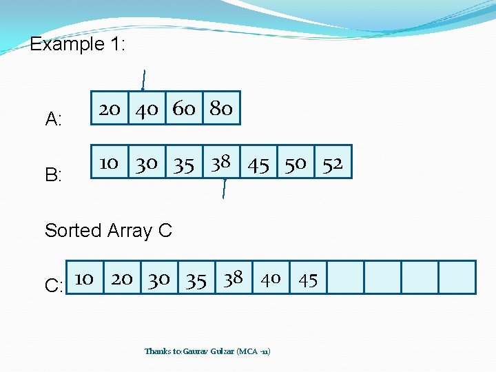
Example 1: A: B: 20 40 60 80 10 30 35 38 45 50 52 Sorted Array C 38 40 45 10 20 30 35 C: Thanks to: Gaurav Gulzar (MCA -11)

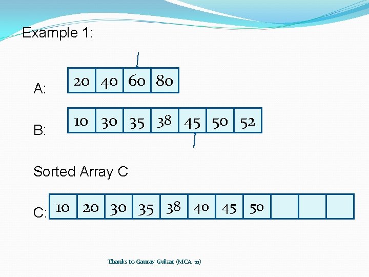
Example 1: A: B: 20 40 60 80 10 30 35 38 45 50 52 Sorted Array C 38 40 45 50 10 20 30 35 C: Thanks to: Gaurav Gulzar (MCA -11)

Example 1: A: B: 20 40 60 80 10 30 35 38 45 50 52 Sorted Array C 38 40 45 50 52 10 20 30 35 C: Thanks to: Gaurav Gulzar (MCA -11)

Example 1: A: B: 20 40 60 80 10 30 35 38 45 50 52 Sorted Array C 38 40 45 50 52 60 80 10 20 30 35 C: Thanks to: Gaurav Gulzar (MCA -11)

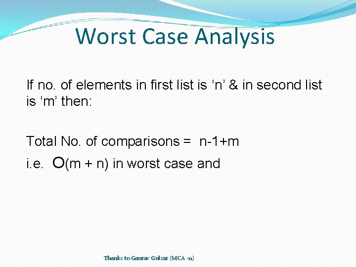
Worst Case Analysis If no. of elements in first list is ‘n’ & in second list is ‘m’ then: Total No. of comparisons = n-1+m i. e. O(m + n) in worst case and Thanks to: Gaurav Gulzar (MCA -11)

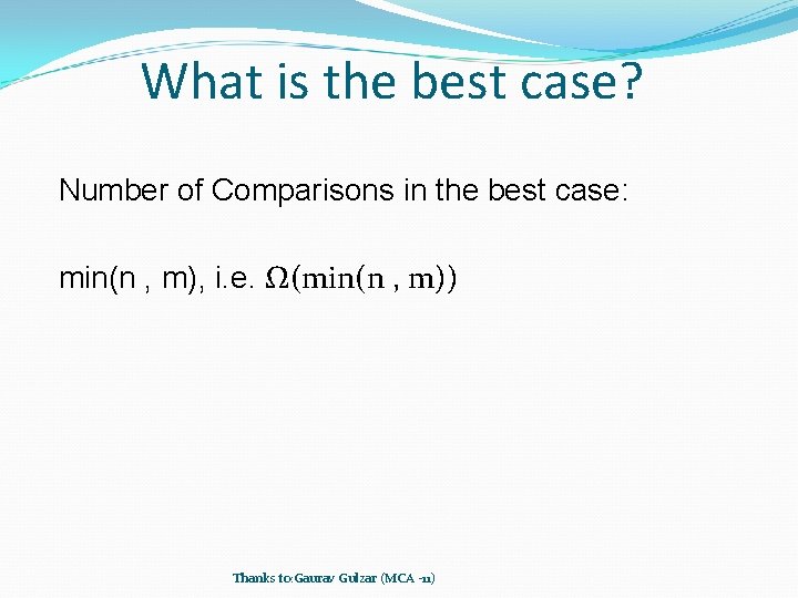
What is the best case? Number of Comparisons in the best case: min(n , m), i. e. Ω(min(n , m)) Thanks to: Gaurav Gulzar (MCA -11)

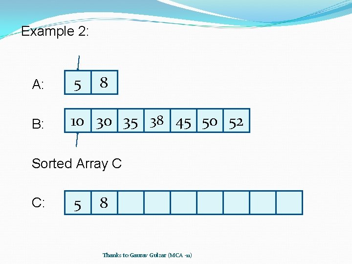
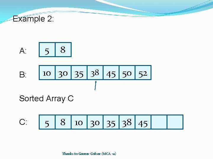
Example 2: A: 5 8 B: 10 30 35 38 45 50 52 Sorted Array C C: 5 8 Thanks to: Gaurav Gulzar (MCA -11)

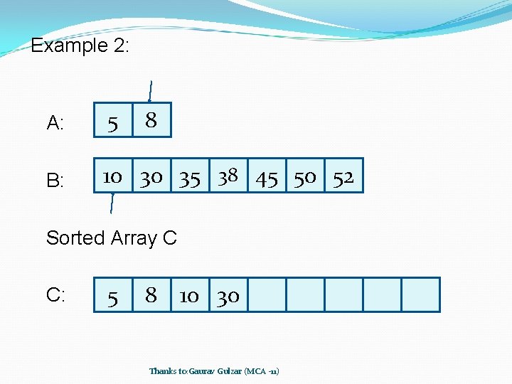
Example 2: A: 5 8 B: 10 30 35 38 45 50 52 Sorted Array C C: 5 8 10 30 Thanks to: Gaurav Gulzar (MCA -11)

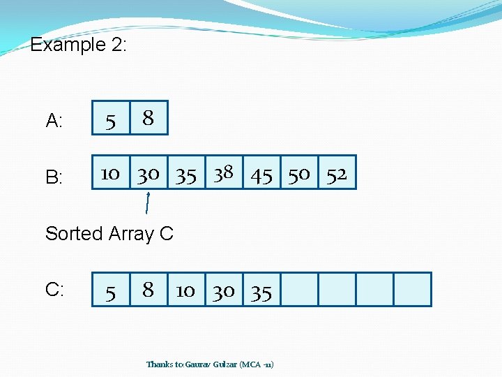
Example 2: A: 5 8 B: 10 30 35 38 45 50 52 Sorted Array C C: 5 8 10 30 35 Thanks to: Gaurav Gulzar (MCA -11)

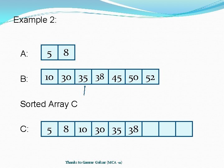
Example 2: A: 5 8 B: 10 30 35 38 45 50 52 Sorted Array C C: 5 8 10 30 35 38 Thanks to: Gaurav Gulzar (MCA -11)

Example 2: A: 5 8 B: 10 30 35 38 45 50 52 Sorted Array C C: 5 8 10 30 35 38 45 Thanks to: Gaurav Gulzar (MCA -11)

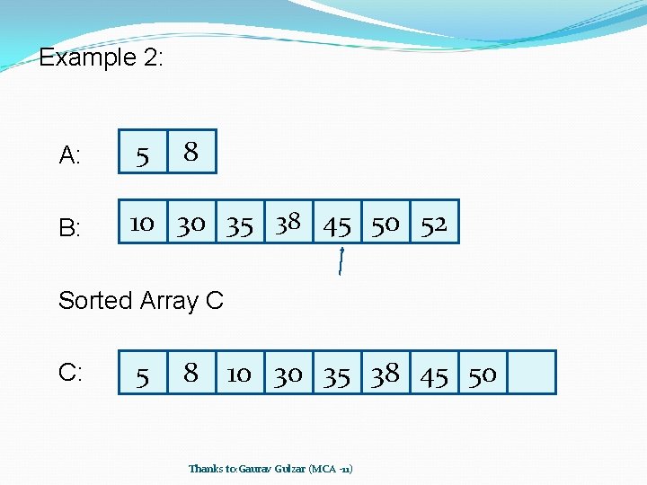
Example 2: A: 5 8 B: 10 30 35 38 45 50 52 Sorted Array C C: 5 8 10 30 35 38 45 50 Thanks to: Gaurav Gulzar (MCA -11)

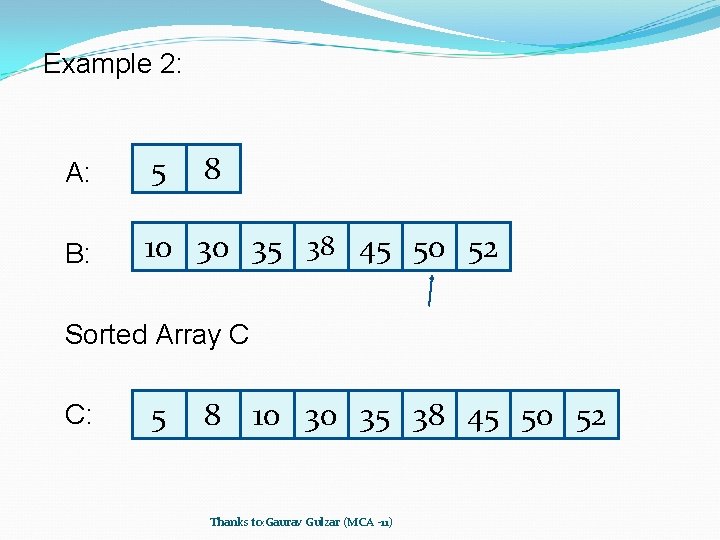
Example 2: A: 5 8 B: 10 30 35 38 45 50 52 Sorted Array C C: 5 8 10 30 35 38 45 50 52 Thanks to: Gaurav Gulzar (MCA -11)

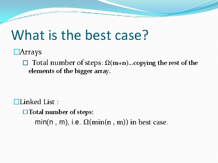
What is the best case? �Arrays � Total number of steps: Ω(m+n)…copying the rest of the elements of the bigger array. �Linked List : �Total number of steps: min(n , m), i. e. Ω(min(n , m)) in best case.

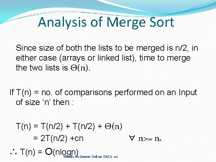
Analysis of Merge Sort Since size of both the lists to be merged is n/2, in either case (arrays or linked list), time to merge the two lists is Θ(n). If T(n) = no. of comparisons performed on an Input of size ‘n’ then : T(n) = T(n/2) + Θ(n) = 2 T(n/2) +cn ∀ n>= n 0 ∴ T(n) = O(nlogn) Thanks to: Gaurav Gulzar (MCA -11)

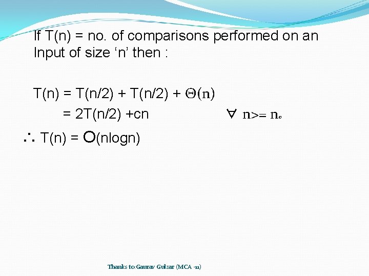
If T(n) = no. of comparisons performed on an Input of size ‘n’ then : T(n) = T(n/2) + Θ(n) = 2 T(n/2) +cn ∀ n>= n 0 ∴ T(n) = O(nlogn) Thanks to: Gaurav Gulzar (MCA -11)

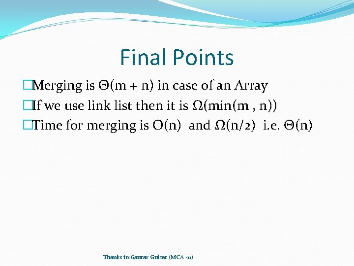
Final Points �Merging is Θ(m + n) in case of an Array �If we use link list then it is Ω(min(m , n)) �Time for merging is O(n) and Ω(n/2) i. e. Θ(n) Thanks to: Gaurav Gulzar (MCA -11)

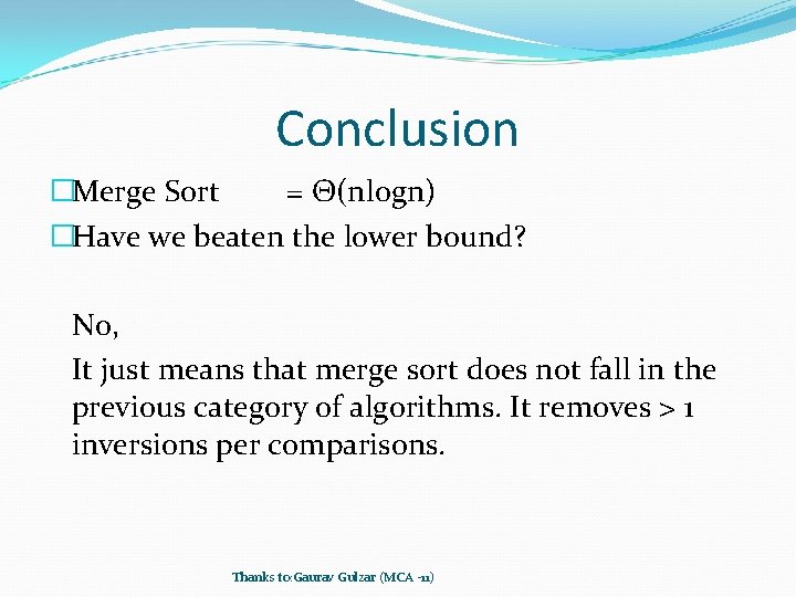
Conclusion �Merge Sort = Θ(nlogn) �Have we beaten the lower bound? No, It just means that merge sort does not fall in the previous category of algorithms. It removes > 1 inversions per comparisons. Thanks to: Gaurav Gulzar (MCA -11)

�What is the �Worst case �Best Case for Merge Sort?

Merge Sort Vs Insertion Sort What is the advantage of merge sort? What is the advantage of insertion sort?

Merge Sort Vs Insertion Sort contd. . �Merge Sort is faster but does not take advantage if the list is already partially sorted. �Insertion Sort takes advantage if the list is already partially sorted.

Lower Bound �Any algorithm that sorts by comparison only does at least (n lg n) comparisons in the worst case.

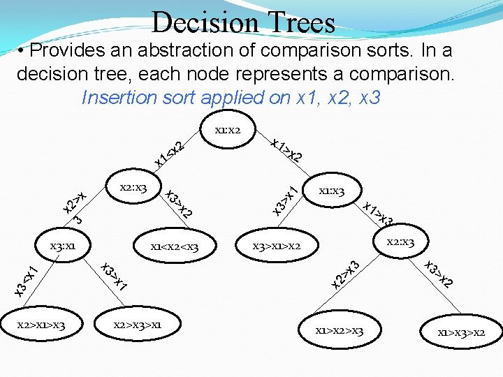
Decision Trees • Provides an abstraction of comparison sorts. In a decision tree, each node represents a comparison. Insertion sort applied on x 1, x 2, x 3 2 >x <x 1 x 3>x 1>x 2 x 3 1 x 3 x 1<x 2<x 3 3 x 3: x 1 x 2>x 1>x 3 >x x 3 x 2 x 3 >x x 2: x 3 >x >x 2 x 2>x 3>x 1 x 1: x 3 x 1 >x 3 x 2: x 3 3 < x 1 x 2 >x x 2 1 x 1: x 2 x 1>x 2>x 3 >x 2 x 1>x 3>x 2

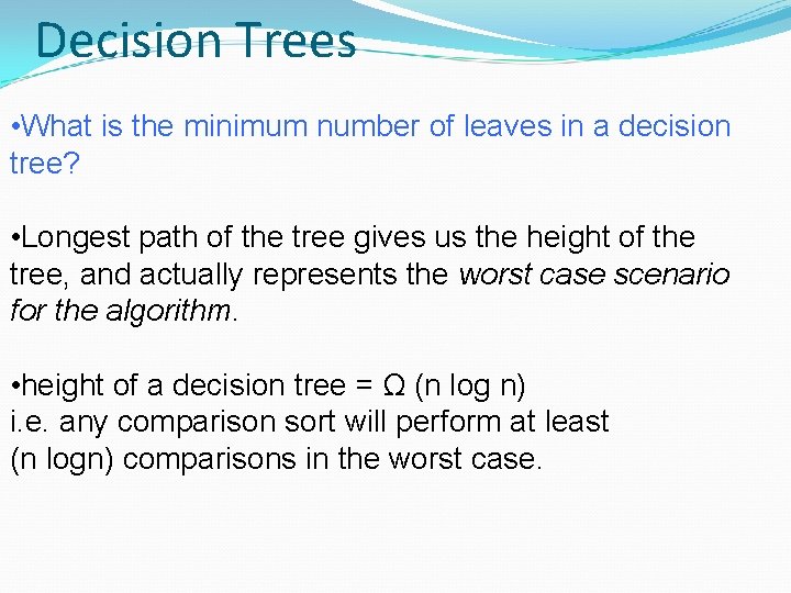
Decision Trees • What is the minimum number of leaves in a decision tree? • Longest path of the tree gives us the height of the tree, and actually represents the worst case scenario for the algorithm. • height of a decision tree = Ω (n log n) i. e. any comparison sort will perform at least (n logn) comparisons in the worst case.

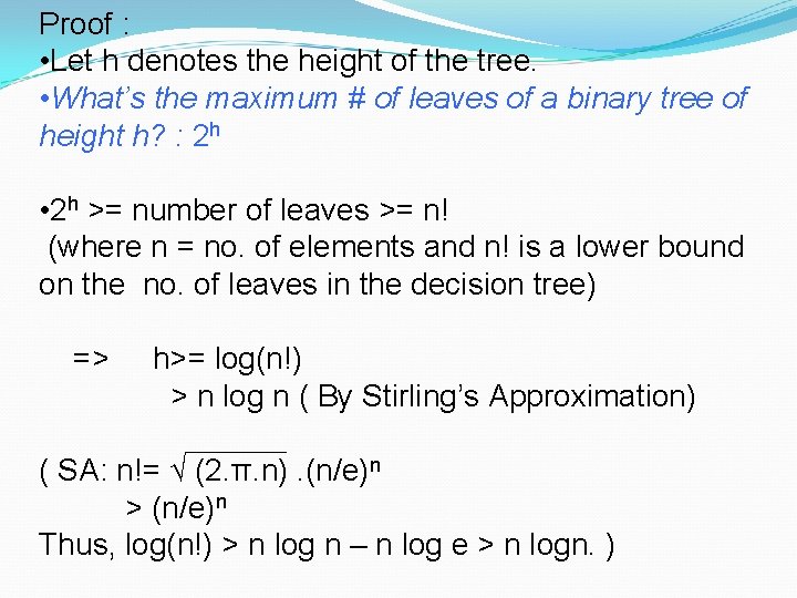
Proof : • Let h denotes the height of the tree. • What’s the maximum # of leaves of a binary tree of height h? : 2 h • 2 h >= number of leaves >= n! (where n = no. of elements and n! is a lower bound on the no. of leaves in the decision tree) => h>= log(n!) > n log n ( By Stirling’s Approximation) ( SA: n!= √ (2. π. n). (n/e)n > (n/e)n Thus, log(n!) > n log n – n log e > n logn. )

Merge Sort is Optimal �Thus the time to comparison sort n elements is (n lg n) �Corollary: Merge-sort is asymptotically optimal comparison sorts. �Later we’ll see another sorting algorithm in this category namely heap-sort that is also optimal. �We’ll also see some algorithms which beat this bound. Needless to say those algorithms are not purely based on comparisons. They do something extra.

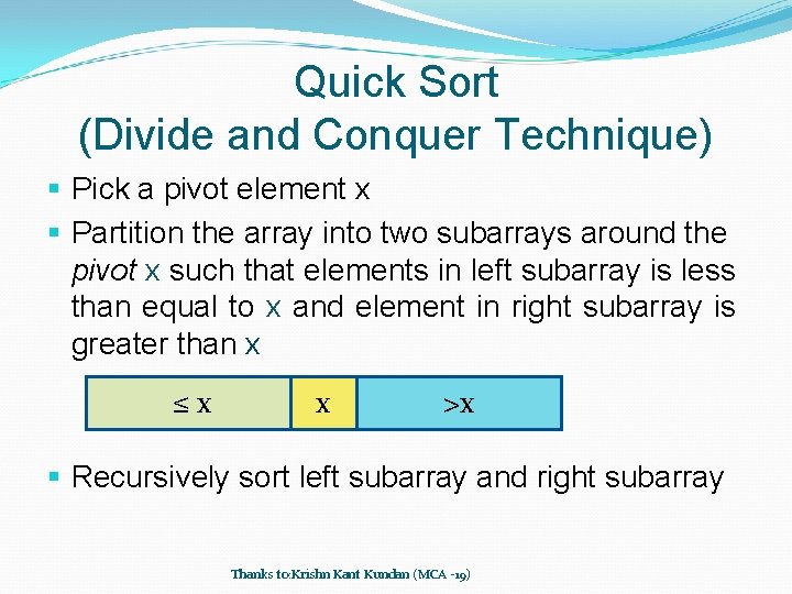
Quick Sort (Divide and Conquer Technique) § Pick a pivot element x § Partition the array into two subarrays around the pivot x such that elements in left subarray is less than equal to x and element in right subarray is greater than x ≤ x x >x § Recursively sort left subarray and right subarray Thanks to: Krishn Kant Kundan (MCA -19)

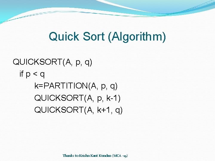
Quick Sort (Algorithm) QUICKSORT(A, p, q) if p < q k=PARTITION(A, p, q) QUICKSORT(A, p, k-1) QUICKSORT(A, k+1, q) Thanks to: Krishn Kant Kundan (MCA -19)

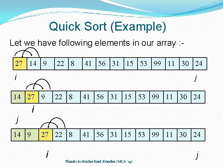
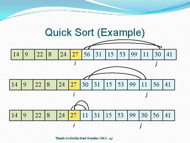
Quick Sort (Example) Let we have following elements in our array : 27 14 9 22 8 41 56 31 15 53 99 11 30 24 i j 14 27 9 j 14 9 22 8 41 56 31 15 53 99 11 30 24 27 22 8 41 56 31 15 53 99 11 30 24 i i Thanks to: Krishn Kant Kundan (MCA -19) j

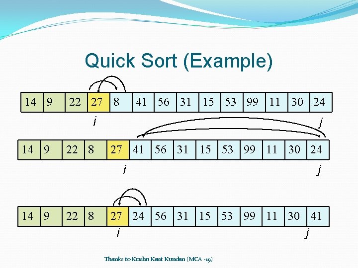
Quick Sort (Example) 14 9 22 27 8 41 56 31 15 53 99 11 30 24 i j 22 8 27 41 56 31 15 53 99 11 30 24 i 14 9 22 8 j 27 24 56 31 15 53 99 11 30 41 i j Thanks to: Krishn Kant Kundan (MCA -19)

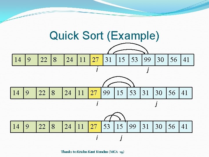
Quick Sort (Example) 14 9 22 8 24 27 56 31 15 53 99 11 30 41 i 14 9 22 8 j 24 27 30 31 15 53 99 11 56 41 i 14 9 22 8 j 24 27 11 31 15 53 99 30 56 41 i Thanks to: Krishn Kant Kundan (MCA -19) j

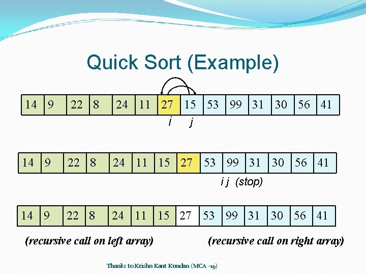
Quick Sort (Example) 14 9 22 8 24 11 27 31 15 53 99 30 56 41 i 14 9 22 8 j 24 11 27 99 15 53 31 30 56 41 i 14 9 22 8 j 24 11 27 53 15 99 31 30 56 41 i j Thanks to: Krishn Kant Kundan (MCA -19)

Quick Sort (Example) 14 9 22 8 24 11 27 15 53 99 31 30 56 41 i 14 9 22 8 j 24 11 15 27 53 99 31 30 56 41 i j (stop) 14 9 22 8 24 11 15 27 53 99 31 30 56 41 (recursive call on left array) (recursive call on right array) Thanks to: Krishn Kant Kundan (MCA -19)

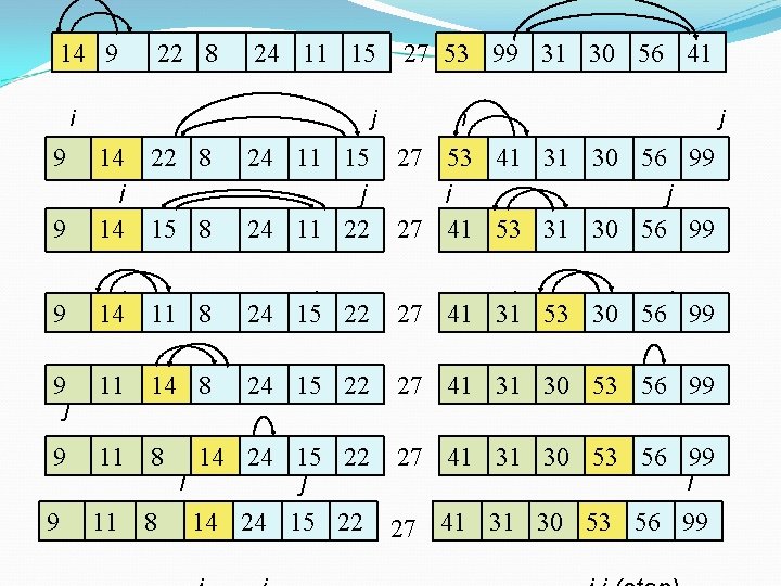
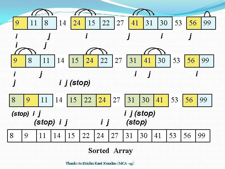
14 9 22 8 24 11 15 i 9 j 27 53 99 31 30 56 41 i 9 14 22 8 i 14 15 8 24 11 15 j 24 11 22 27 53 41 31 30 56 99 i j 27 41 53 31 30 56 99 9 14 i 11 8 24 15 j 22 27 41 31 i 53 30 56 j 99 9 j i 14 8 11 j 15 22 24 27 41 31 30 i 53 56 99 9 11 8 14 24 15 22 i j 27 41 31 30 53 56 99 i 9 j 11 8 14 24 15 22 27 41 31 30 53 56 99 j

9 11 8 j i i i j 8 j 11 14 15 24 22 27 31 41 30 53 56 99 j i j i i j (stop) 9 11 14 15 22 24 27 31 30 41 53 56 99 j (stop) i 8 i j 9 8 14 24 15 22 27 41 31 30 53 56 99 9 i j (stop) 11 14 15 22 24 27 31 30 41 53 56 99 Sorted Array Thanks to: Krishn Kant Kundan (MCA -19)

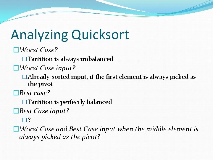
Analyzing Quicksort �Worst Case? �Partition is always unbalanced �Worst Case input? �Already-sorted input, if the first element is always picked as the pivot �Best case? �Partition is perfectly balanced �Best Case input? �? �Worst Case and Best Case input when the middle element is always picked as the pivot?

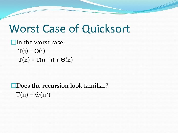
Worst Case of Quicksort �In the worst case: T(1) = (1) T(n) = T(n - 1) + (n) �Does the recursion look familiar? T(n) = (n 2)

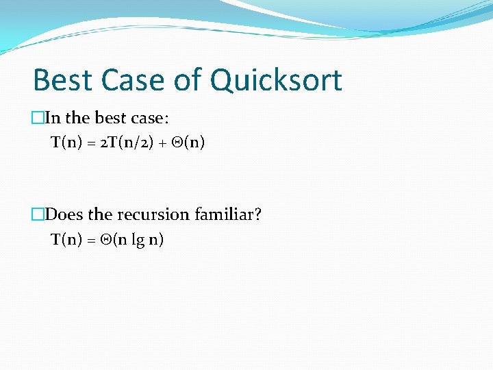
Best Case of Quicksort �In the best case: T(n) = 2 T(n/2) + (n) �Does the recursion familiar? T(n) = (n lg n)

Why does Qsort works well in practice? �Suppose that partition() always produces a 9 -to-1 split. This looks quite unbalanced! �The recurrence is: T(n) = T(9 n/10) + T(n/10) + n �T(n) = θ (n log n) �Such an imbalanced partition and θ(n log n) time?

Why does Qsort works well in practice? �Intuitively, a real-life run of quicksort will produce a mix of “bad” and “good” splits �Pretend for intuition that they alternate between bestcase (n/2 : n/2) and worst-case (n-1 : 1) �What happens if we bad-split root node, then good-split the resulting size (n-1) node?

Why does Qsort works well in practice? �Intuitively, a real-life run of quicksort will produce a mix of “bad” and “good” splits �Pretend for intuition that they alternate between best- case (n/2 : n/2) and worst-case (n-1 : 1) �What happens if we bad-split root node, then good-split the resulting size (n-1) node? We end up with three subarrays, size 1, (n-1)/2 � Combined cost of splits = n + n -1 = 2 n -1 = O(n) � No worse than if we had good-split the root node! �

Why does Qsort works well in practice? �Intuitively, the O(n) cost of a bad split (or 2 or 3 bad splits) can be absorbed into the O(n) cost of each good split �Thus running time of alternating bad and good splits is still O(n lg n), with slightly higher constants �How can we be more rigorous? : we’ll do average analysis of Qsort later while doing randomized algorithms.

Quicksort Vs Merge Sort �Merge Sort takes O(n lg n) in the worst case �Quick Sort takes O(n 2) in the worst case �So why would anybody use Qsort instead of merge sort? �Because in practice, Qsort is quick as the worst case doesn’t happen often.

Up Next Linear-Time Sorting Algorithms

The End