Mocha jl Deep Learning for Julia Chiyuan Zhang

Mocha. jl Deep Learning for Julia Chiyuan Zhang (@pluskid) CSAIL, MIT

JULIA BASICS 10 -minute Introduction to Julia

A glance of basic syntax Numpy Matlab Julia Description x[0] x(1) x[1] Index 1 st elem of array np. random. randn(3, 3) 3 -by-3 random Gaussian matrix np. arange(1, 11) 1: 10 1, 2, …, 10 X*Y X. * Y Elementwise mul np. dot(X, Y) X*Y Matrix mul linalg. solve(X, Y) XY Left matrix division d = {‘one’: 1, ‘two’: 2} d[‘one’] d = containers. Map({‘one’, ’two’}, {1, 2}); d(‘one’) d = Dict("one"=>1, "two"=>2) d["one"] Hash table r = np. random. rand(*x. shape) y = x * (r > t) r = rand(size(x)) y = x. * (r. > t) Dropout f = lambda x, mu, sigma: np. exp(-(xmu)**2/(2*sigma**2)) / sqrt(2*np. pi*sigma^2) f=@(x, mu, sigma) exp(-(x-mu)^2/(2*sigma^2)) / sqrt(2*pi*sigma^2) f(x, μ, �� )= exp(-(x-μ)^2/2�� ^2)/sqrt(2π*�� ^2) Gaussian density function

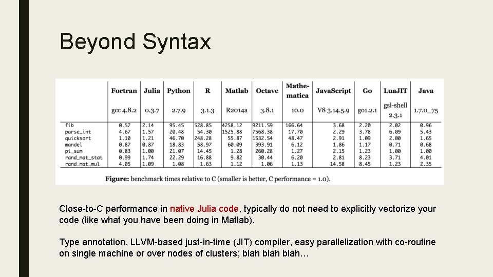
Beyond Syntax Close-to-C performance in native Julia code, typically do not need to explicitly vectorize your code (like what you have been doing in Matlab). Type annotation, LLVM-based just-in-time (JIT) compiler, easy parallelization with co-routine on single machine or over nodes of clusters; blah…

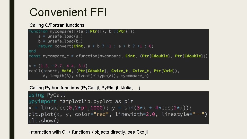
Convenient FFI Calling C/Fortran functions Calling Python functions (Py. Call. jl, Py. Plot. jl, IJulia, …) Interaction with C++ functions / objects directly, see Cxx. jl

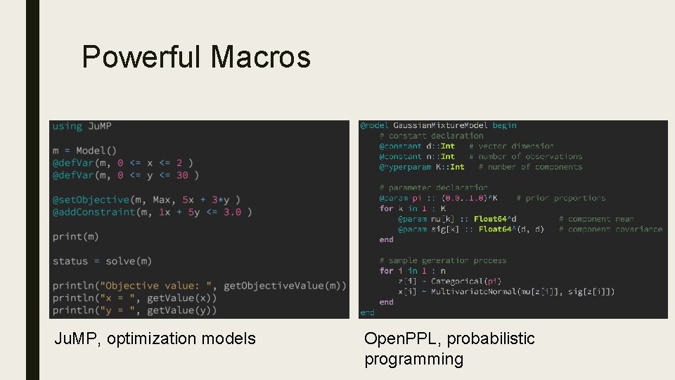
Powerful Macros Ju. MP, optimization models Open. PPL, probabilistic programming

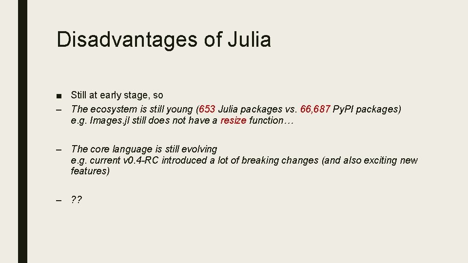
Disadvantages of Julia ■ Still at early stage, so – The ecosystem is still young (653 Julia packages vs. 66, 687 Py. PI packages) e. g. Images. jl still does not have a resize function… – The core language is still evolving e. g. current v 0. 4 -RC introduced a lot of breaking changes (and also exciting new features) – ? ?

MOCHA. JL Deep Learning in Julia

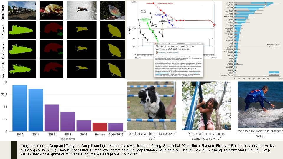
Image sources: Li Deng and Dong Yu. Deep Learning – Methods and Applications. Zheng, Shuai et al. “Conditional Random Fields as Recurrent Neural Networks. ” ar. Xiv. org cs. CV (2015). Google Deep Mind. Human-level control through deep reinforcement learning. Nature, Feb. 2015. Andrej Karpathy and Li Fei-Fei. Deep Visual-Semantic Alignments for Generating Image Descriptions. CVPR 2015.

Why Deep Learning is Successful? ■ Theoretical point of view – Nowhere near a complete theoretical understanding of deep learning yet ■ Practical point of view – Big Data: large amount of (thank Internet) labeled (thank Amazon M-Turk), high -dimensional (large images, videos, speech and text corpus, etc. ) – Computational Power: GPUs, large clusters – Human Power: the “deep learning conspiracy” – Software Engineering: network architecture & computation components decoupled

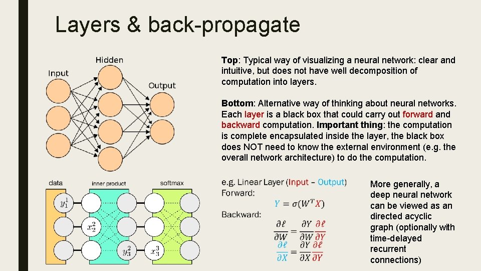
Layers & back-propagate Top: Typical way of visualizing a neural network: clear and intuitive, but does not have well decomposition of computation into layers. Bottom: Alternative way of thinking about neural networks. Each layer is a black box that could carry out forward and backward computation. Important thing: the computation is complete encapsulated inside the layer, the black box does NOT need to know the external environment (e. g. the overall network architecture) to do the computation. More generally, a deep neural network can be viewed as an directed acyclic graph (optionally with time-delayed recurrent connections)

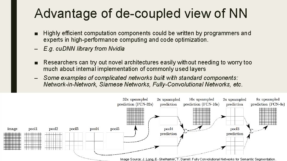
Advantage of de-coupled view of NN ■ Highly efficient computation components could be written by programmers and experts in high-performance computing and code optimization. – E. g. cu. DNN library from Nvidia ■ Researchers can try out novel architectures easily without needing to worry too much about internal implementation of commonly used layers – Some examples of complicated networks built with standard components: Network-in-Network, Siamese Networks, Fully-Convolutional Networks, etc. Image Source: J. Long, E. Shelhamer, T. Darrell. Fully Convolutional Networks for Semantic Segmentation.

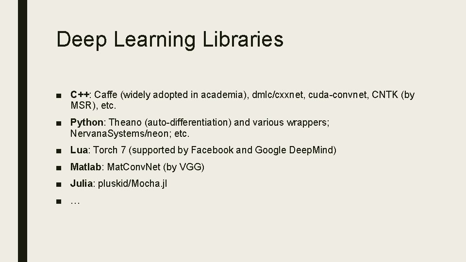
Deep Learning Libraries ■ C++: Caffe (widely adopted in academia), dmlc/cxxnet, cuda-convnet, CNTK (by MSR), etc. ■ Python: Theano (auto-differentiation) and various wrappers; Nervana. Systems/neon; etc. ■ Lua: Torch 7 (supported by Facebook and Google Deep. Mind) ■ Matlab: Mat. Conv. Net (by VGG) ■ Julia: pluskid/Mocha. jl ■ …

Why Mocha. jl? 1. Julia: written in Julia and easy interaction with the rest of the Julia ecosystem. 2. Minimum dependency: the Julia backend runs out of the box. CUDA backend depends on Nvidia cu. DNN. 3. Correctness: all the computation components are unit-tested. 4. Modular architecture: layers, activation functions, regularizers, network topology, solvers, etc. Julia compiles with LLVM, so potentially Julia code could be compiled directly to GPU devices in the future. After that, writing neural networks in Julia will be really enjoyable!

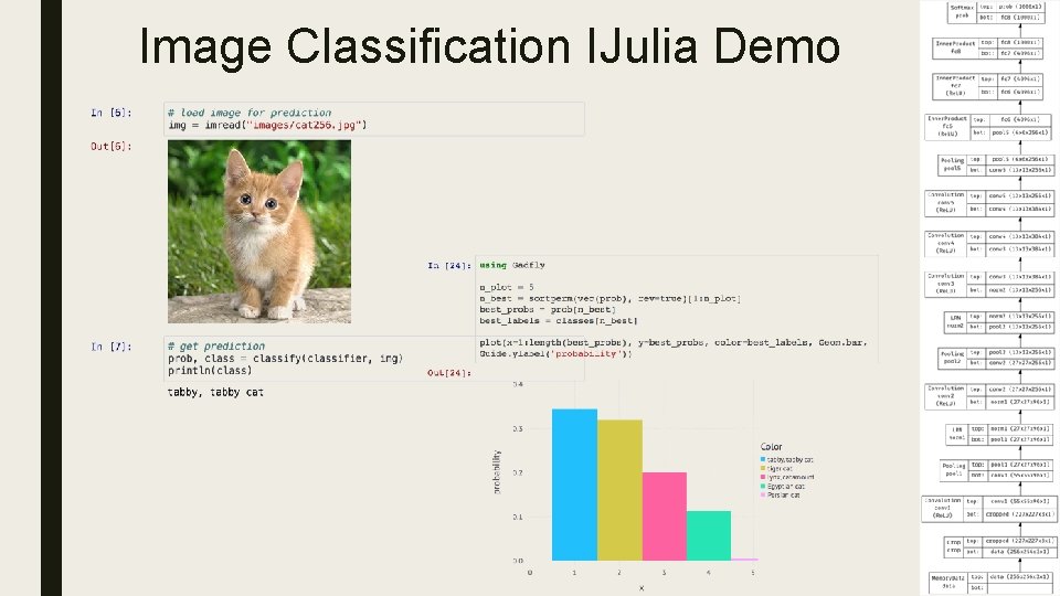
Image Classification IJulia Demo

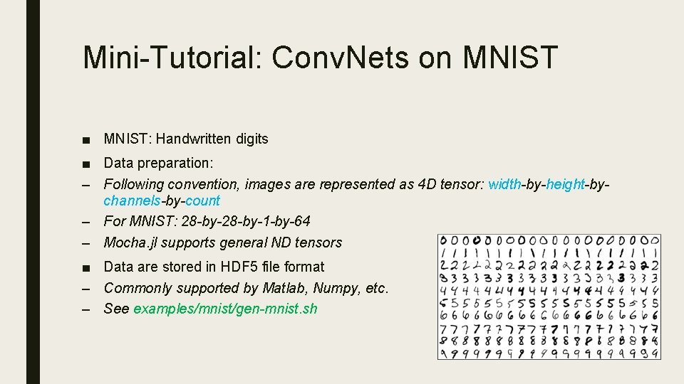
Mini-Tutorial: Conv. Nets on MNIST ■ MNIST: Handwritten digits ■ Data preparation: – Following convention, images are represented as 4 D tensor: width-by-height-bychannels-by-count – For MNIST: 28 -by-1 -by-64 – Mocha. jl supports general ND tensors ■ Data are stored in HDF 5 file format – Commonly supported by Matlab, Numpy, etc. – See examples/mnist/gen-mnist. sh

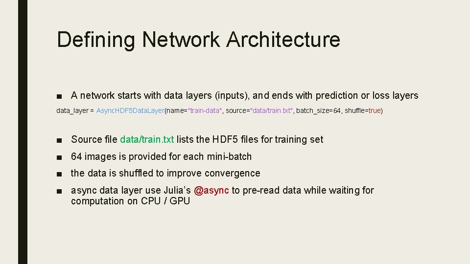
Defining Network Architecture ■ A network starts with data layers (inputs), and ends with prediction or loss layers data_layer = Async. HDF 5 Data. Layer(name="train-data", source="data/train. txt", batch_size=64, shuffle=true) ■ Source file data/train. txt lists the HDF 5 files for training set ■ 64 images is provided for each mini-batch ■ the data is shuffled to improve convergence ■ async data layer use Julia’s @async to pre-read data while waiting for computation on CPU / GPU

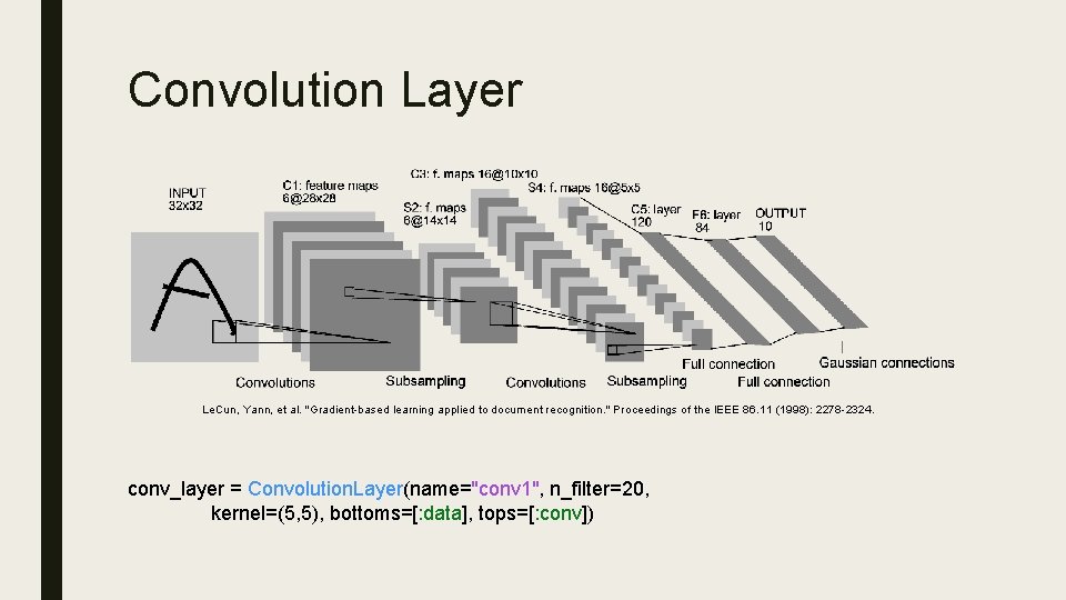
Convolution Layer Le. Cun, Yann, et al. "Gradient-based learning applied to document recognition. " Proceedings of the IEEE 86. 11 (1998): 2278 -2324. conv_layer = Convolution. Layer(name="conv 1", n_filter=20, kernel=(5, 5), bottoms=[: data], tops=[: conv])

Pooling Layer pool_layer = Pooling. Layer(name="pool 1", kernel=(2, 2), stride=(2, 2), bottoms=[: conv], tops=[: pool]) ■ Pooling layer operate on the output of convolution layer ■ By default, MAX pooling is performed; can switch to MEAN pooling by specifying pooling=Pooling. Mean()

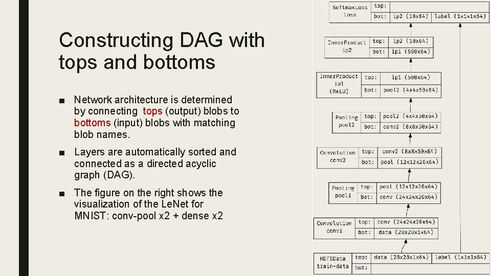
Constructing DAG with tops and bottoms ■ Network architecture is determined by connecting tops (output) blobs to bottoms (input) blobs with matching blob names. ■ Layers are automatically sorted and connected as a directed acyclic graph (DAG). ■ The figure on the right shows the visualization of the Le. Net for MNIST: conv-pool x 2 + dense x 2

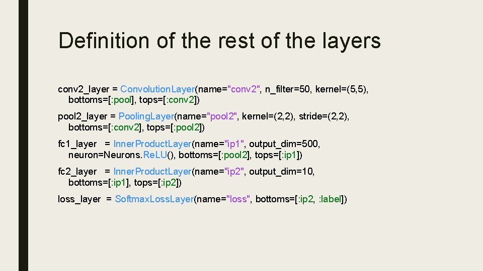
Definition of the rest of the layers conv 2_layer = Convolution. Layer(name="conv 2", n_filter=50, kernel=(5, 5), bottoms=[: pool], tops=[: conv 2]) pool 2_layer = Pooling. Layer(name="pool 2", kernel=(2, 2), stride=(2, 2), bottoms=[: conv 2], tops=[: pool 2]) fc 1_layer = Inner. Product. Layer(name="ip 1", output_dim=500, neuron=Neurons. Re. LU(), bottoms=[: pool 2], tops=[: ip 1]) fc 2_layer = Inner. Product. Layer(name="ip 2", output_dim=10, bottoms=[: ip 1], tops=[: ip 2]) loss_layer = Softmax. Loss. Layer(name="loss", bottoms=[: ip 2, : label])

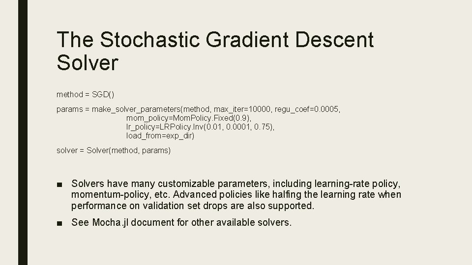
The Stochastic Gradient Descent Solver method = SGD() params = make_solver_parameters(method, max_iter=10000, regu_coef=0. 0005, mom_policy=Mom. Policy. Fixed(0. 9), lr_policy=LRPolicy. Inv(0. 01, 0. 0001, 0. 75), load_from=exp_dir) solver = Solver(method, params) ■ Solvers have many customizable parameters, including learning-rate policy, momentum-policy, etc. Advanced policies like halfing the learning rate when performance on validation set drops are also supported. ■ See Mocha. jl document for other available solvers.

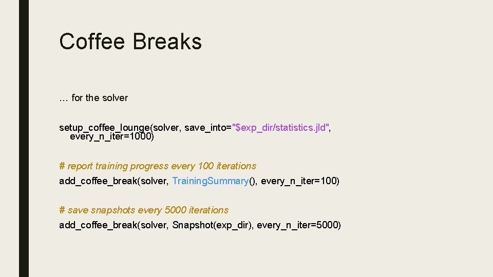
Coffee Breaks … for the solver setup_coffee_lounge(solver, save_into="$exp_dir/statistics. jld", every_n_iter=1000) # report training progress every 100 iterations add_coffee_break(solver, Training. Summary(), every_n_iter=100) # save snapshots every 5000 iterations add_coffee_break(solver, Snapshot(exp_dir), every_n_iter=5000)

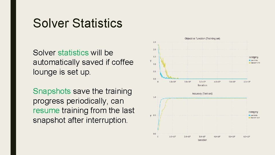
Solver Statistics Solver statistics will be automatically saved if coffee lounge is set up. Snapshots save the training progress periodically, can resume training from the last snapshot after interruption.

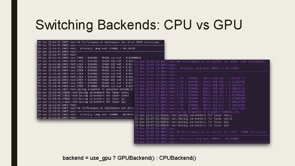
Switching Backends: CPU vs GPU backend = use_gpu ? GPUBackend() : CPUBackend()

THANK YOU! http: //julialang. org https: //github. com/pluskid/Mocha. jl