MIT 3 022 Microstructural Evolution in Materials 3

MIT 3. 022 Microstructural Evolution in Materials 3: Canonical Ensemble Juejun (JJ) Hu hujuejun@mit. edu

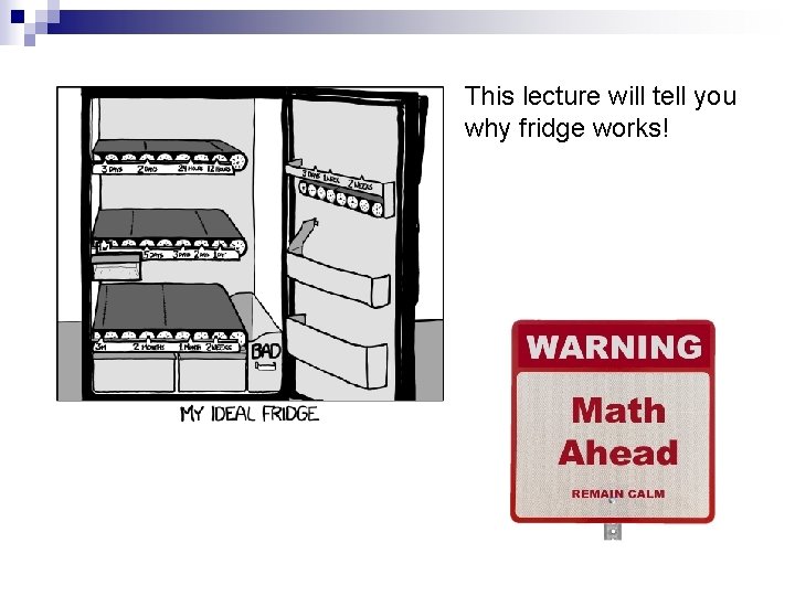
This lecture will tell you why fridge works!

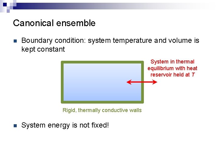
Canonical ensemble n Boundary condition: system temperature and volume is kept constant System in thermal equilibrium with heat reservoir held at T Rigid, thermally conductive walls n System energy is not fixed!

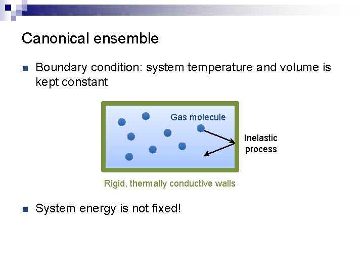
Canonical ensemble n Boundary condition: system temperature and volume is kept constant Gas molecule Inelastic process Rigid, thermally conductive walls n System energy is not fixed!

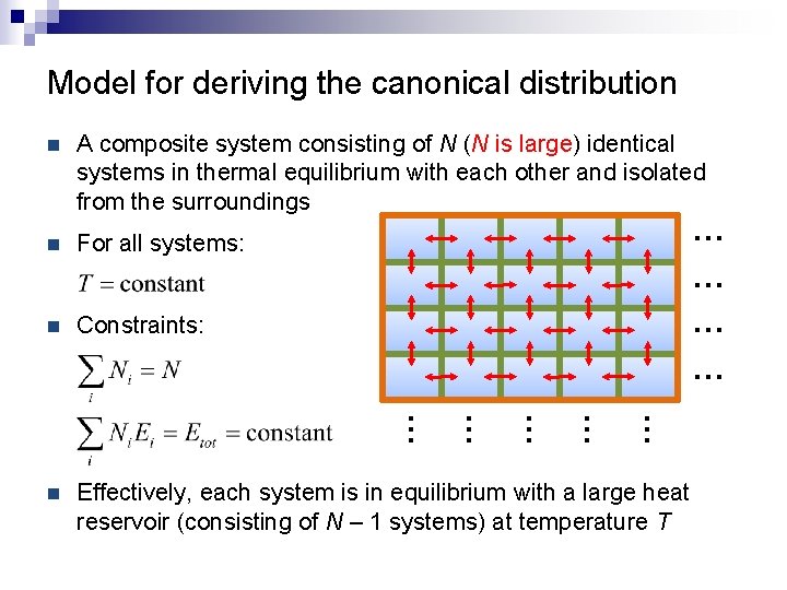
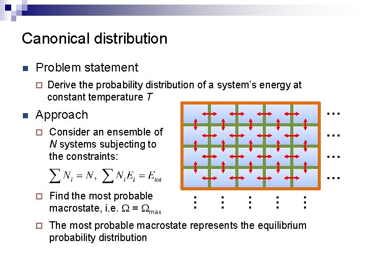
Model for deriving the canonical distribution n A composite system consisting of N (N is large) identical systems in thermal equilibrium with each other and isolated from the surroundings n For all systems: n Constraints: n Effectively, each system is in equilibrium with a large heat reservoir (consisting of N – 1 systems) at temperature T … … … … …

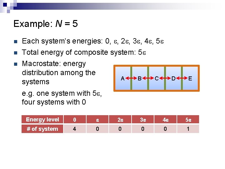
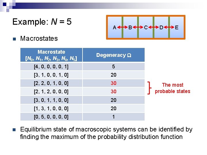
Example: N = 5 n Each system’s energies: 0, e, 2 e, 3 e, 4 e, 5 e n Total energy of composite system: 5 e Macrostate: energy distribution among the A B systems n C D E e. g. one system with 5 e, four systems with 0 Energy level 0 e 2 e 3 e 4 e 5 e # of system 4 0 0 1

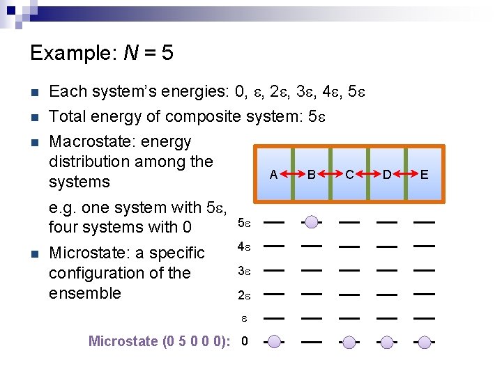
Example: N = 5 n Each system’s energies: 0, e, 2 e, 3 e, 4 e, 5 e n Total energy of composite system: 5 e Macrostate: energy distribution among the A B systems n e. g. one system with 5 e, four systems with 0 n Microstate: a specific configuration of the ensemble 5 e 4 e 3 e 2 e e Microstate (5 0 0): 0 C D E

Example: N = 5 n Each system’s energies: 0, e, 2 e, 3 e, 4 e, 5 e n Total energy of composite system: 5 e Macrostate: energy distribution among the A B systems n e. g. one system with 5 e, four systems with 0 n Microstate: a specific configuration of the ensemble 5 e 4 e 3 e 2 e e Microstate (0 5 0 0 0): 0 C D E

Example: N = 5 n n A B C D E Macrostate Energy level 0 e 2 e 3 e 4 e 5 e # of system 4 0 0 1 Microstates: (5 0 0), (0 5 0 0 0), (0 0 5 0 0), (0 0 0 5 0), (0 0 5) n Number of microstates: W = 5

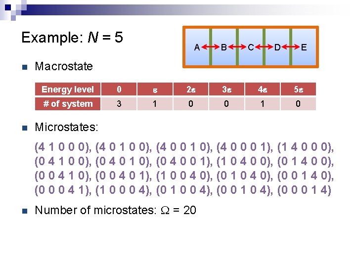
Example: N = 5 n n A B C D E Macrostate Energy level 0 e 2 e 3 e 4 e 5 e # of system 3 1 0 0 1 0 Microstates: (4 1 0 0 0), (4 0 1 0 0), (4 0 0 1 0), (4 0 0 0 1), (1 4 0 0 0), (0 4 1 0 0), (0 4 0 1 0), (0 4 0 0 1), (1 0 4 0 0), (0 1 4 0 0), (0 0 4 1 0), (0 0 4 0 1), (1 0 0 4 0), (0 1 0 4 0), (0 0 1 4 0), (0 0 0 4 1), (1 0 0 0 4), (0 1 0 0 4), (0 0 1 0 4), (0 0 0 1 4) n Number of microstates: W = 20

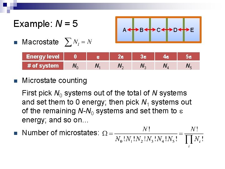
Example: N = 5 n n A B C D E Macrostate Energy level 0 e 2 e 3 e 4 e 5 e # of system N 0 N 1 N 2 N 3 N 4 N 5 Microstate counting First pick N 0 systems out of the total of N systems and set them to 0 energy; then pick N 1 systems out of the remaining N-N 0 systems and set them to e energy; and so on… n Number of microstates:

Example: N = 5 n n A B C D E Macrostates Macrostate [N 0, N 1, N 2, N 3, N 4, N 5] Degeneracy W [4, 0, 0, 1] 5 [3, 1, 0, 0, 1, 0] 20 [2, 2, 0, 1, 0, 0] 30 [2, 1, 2, 0, 0, 0] 30 [3, 0, 1, 1, 0, 0] 20 [1, 3, 1, 0, 0, 0] 20 [0, 5, 0, 0] 1 The most probable states Equilibrium state of macroscopic systems can be identified by finding the maximum of the probability distribution function

Example: N = 5 Small N: broad distribution [400001] [310010] [220100] [212000] [301100] [131000] [050000] Macrostates

Canonical distribution n Problem statement ¨ n Derive the probability distribution of a system’s energy at constant temperature T Approach The most probable macrostate represents the equilibrium probability distribution … ¨ … Find the most probable macrostate, i. e. W = Wmax … ¨ … Consider an ensemble of N systems subjecting to the constraints: … ¨ … …

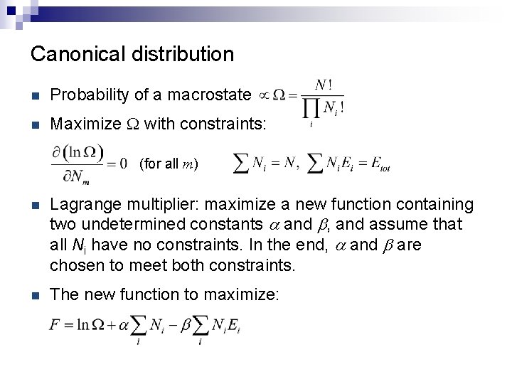
Canonical distribution n Probability of a macrostate n Maximize W with constraints: (for all m) n Lagrange multiplier: maximize a new function containing two undetermined constants a and b, and assume that all Ni have no constraints. In the end, a and b are chosen to meet both constraints. n The new function to maximize:

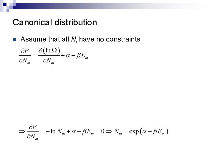
Canonical distribution n Assume that all Ni have no constraints

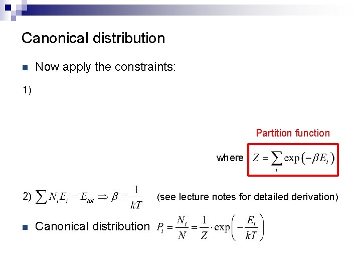
Canonical distribution n Now apply the constraints: 1) Partition function where 2) n (see lecture notes for detailed derivation) Canonical distribution

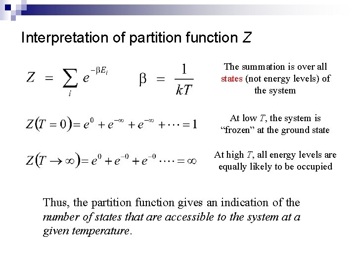
Interpretation of partition function Z The summation is over all states (not energy levels) of the system At low T, the system is “frozen” at the ground state At high T, all energy levels are equally likely to be occupied Thus, the partition function gives an indication of the number of states that are accessible to the system at a given temperature.

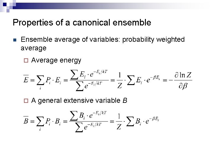
Properties of a canonical ensemble n Ensemble average of variables: probability weighted average ¨ Average energy ¨ A general extensive variable B

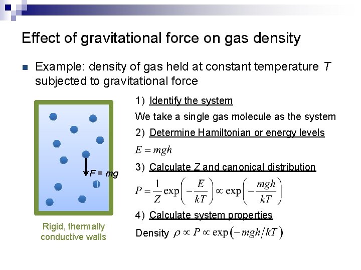
Effect of gravitational force on gas density n Example: density of gas held at constant temperature T subjected to gravitational force 1) Identify the system We take a single gas molecule as the system 2) Determine Hamiltonian or energy levels F = mg 3) Calculate Z and canonical distribution 4) Calculate system properties Rigid, thermally conductive walls Density

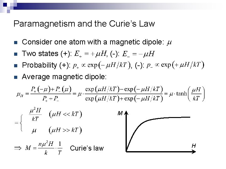
Paramagnetism and the Curie’s Law n Consider one atom with a magnetic dipole: n Two states (+): n Probability (+): n Average magnetic dipole: , (-): M Curie’s law H

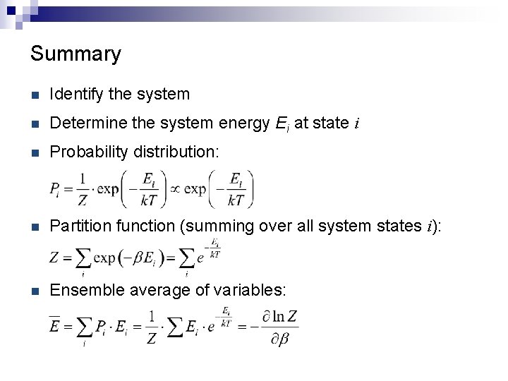
Summary n Identify the system n Determine the system energy Ei at state i n Probability distribution: n Partition function (summing over all system states i): n Ensemble average of variables:

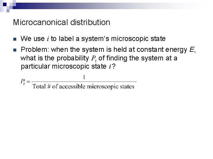
Microcanonical distribution n We use i to label a system’s microscopic state n Problem: when the system is held at constant energy E, what is the probability Pi of finding the system at a particular microscopic state i ?

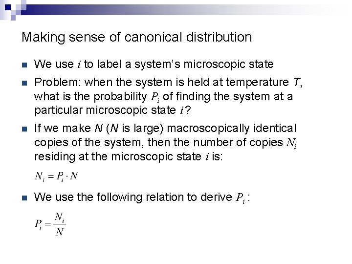
Making sense of canonical distribution n We use i to label a system’s microscopic state n Problem: when the system is held at temperature T, what is the probability Pi of finding the system at a particular microscopic state i ? n If we make N (N is large) macroscopically identical copies of the system, then the number of copies Ni residing at the microscopic state i is: n We use the following relation to derive Pi :

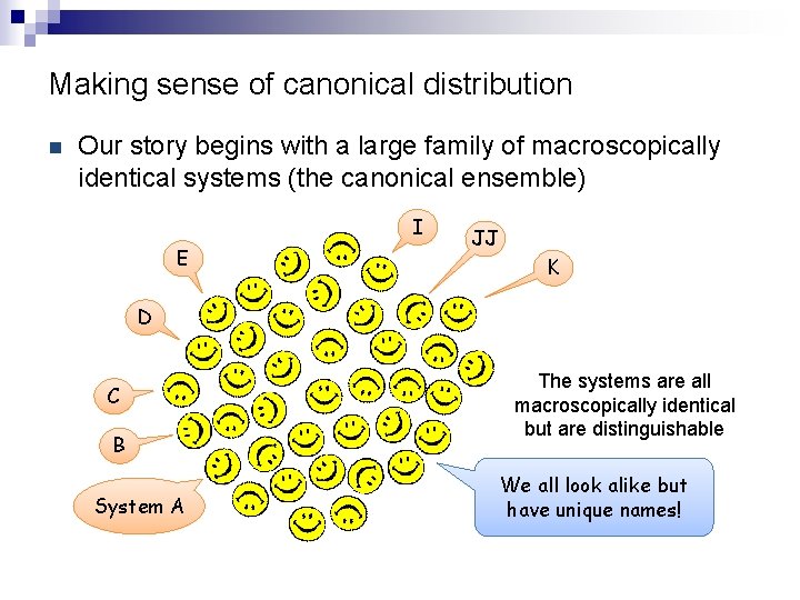
Making sense of canonical distribution n Our story begins with a large family of macroscopically identical systems (the canonical ensemble) I E JJ K D C B System A The systems are all macroscopically identical but are distinguishable We all look alike but have unique names!

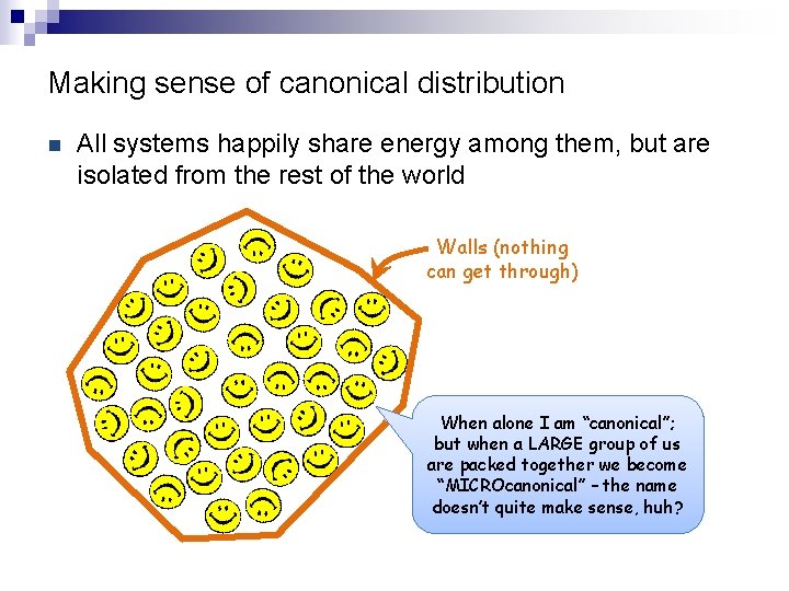
Making sense of canonical distribution n All systems happily share energy among them, but are isolated from the rest of the world Walls (nothing can get through) When alone I am “canonical”; but when a LARGE group of us are packed together we become “MICROcanonical” – the name doesn’t quite make sense, huh?

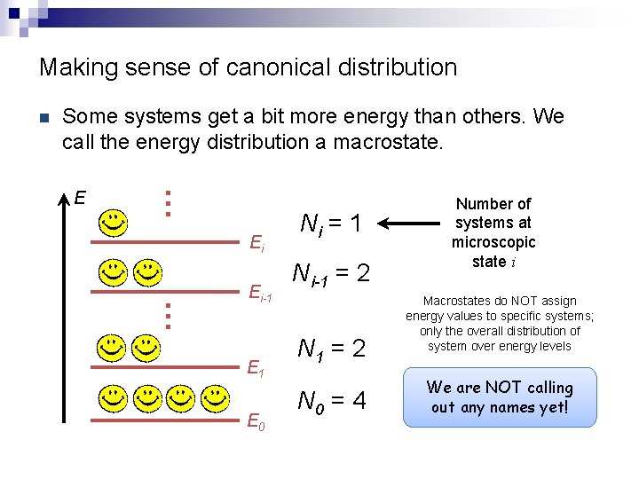
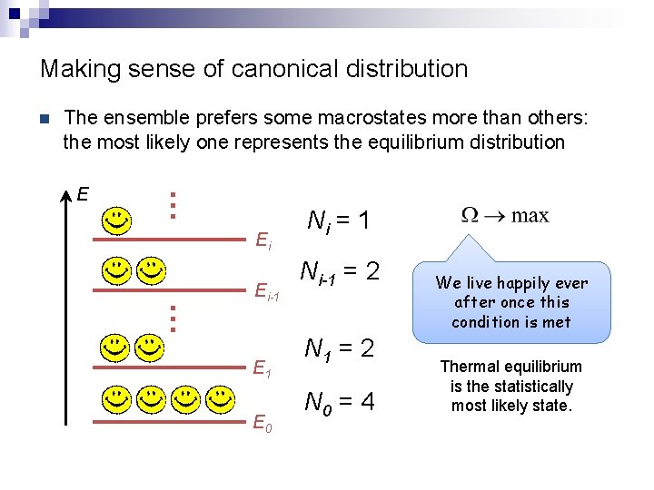
Making sense of canonical distribution E … Some systems get a bit more energy than others. We call the energy distribution a macrostate. Ei … n Ei-1 E 0 Ni = 1 Ni-1 = 2 N 0 = 4 Number of systems at microscopic state i Macrostates do NOT assign energy values to specific systems; only the overall distribution of system over energy levels We are NOT calling out any names yet!

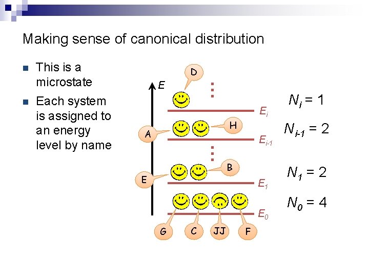
Making sense of canonical distribution Each system is assigned to an energy level by name D E … n This is a microstate Ei H A … n E Ei-1 B E 1 E 0 G C JJ F Ni = 1 Ni-1 = 2 N 0 = 4

Making sense of canonical distribution E … The ensemble prefers some macrostates more than others: the most likely one represents the equilibrium distribution Ei … n Ei-1 E 0 Ni = 1 Ni-1 = 2 N 0 = 4 We live happily ever after once this condition is met Thermal equilibrium is the statistically most likely state.

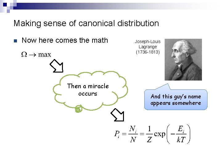
Making sense of canonical distribution n Now here comes the math Then a miracle occurs Joseph-Louis Lagrange (1736 -1813) And this guy’s name appears somewhere

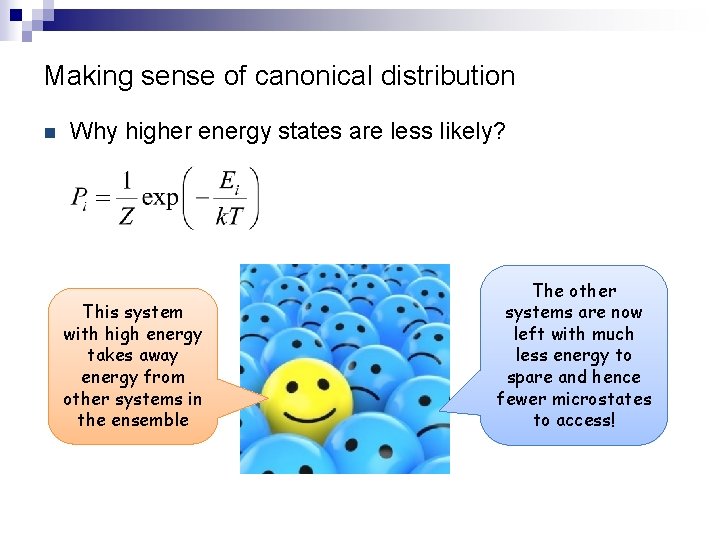
Making sense of canonical distribution n Why higher energy states are less likely? This system with high energy takes away energy from other systems in the ensemble The other systems are now left with much less energy to spare and hence fewer microstates to access!

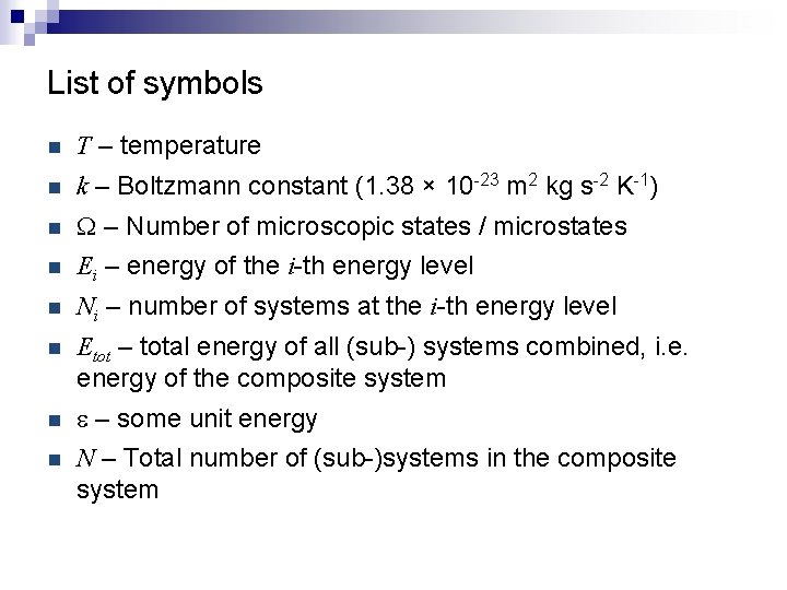
List of symbols n T – temperature n k – Boltzmann constant (1. 38 × 10 -23 m 2 kg s-2 K-1) n W – Number of microscopic states / microstates n Ei – energy of the i-th energy level n Ni – number of systems at the i-th energy level n Etot – total energy of all (sub-) systems combined, i. e. energy of the composite system n e – some unit energy n N – Total number of (sub-)systems in the composite system

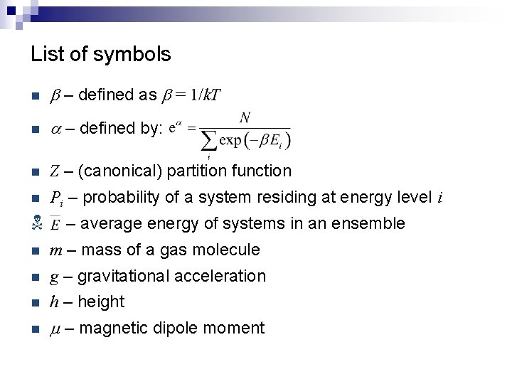
List of symbols n b – defined as b = 1/k. T n a – defined by: n Z – (canonical) partition function n Pi – probability of a system residing at energy level i N – average energy of systems in an ensemble n m – mass of a gas molecule n g – gravitational acceleration n h – height n m – magnetic dipole moment

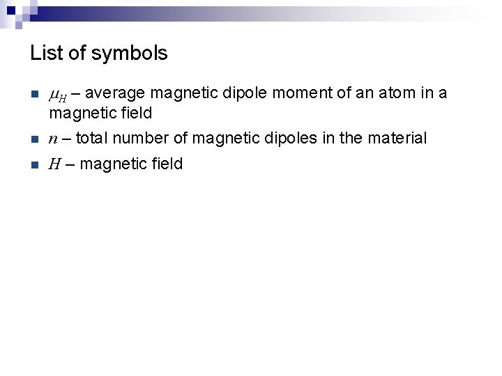
List of symbols n m. H – average magnetic dipole moment of an atom in a magnetic field n n – total number of magnetic dipoles in the material n H – magnetic field