Memorial University of Newfoundland Faculty of Engineering Applied

Memorial University of Newfoundland Faculty of Engineering & Applied Science Engineering 7854 Industrial Machine Vision INTRODUCTION TO MACHINE VISION Prof. Nick Krouglicof

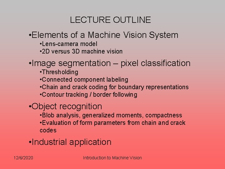
LECTURE OUTLINE • Elements of a Machine Vision System • Lens-camera model • 2 D versus 3 D machine vision • Image segmentation – pixel classification • Thresholding • Connected component labeling • Chain and crack coding for boundary representations • Contour tracking / border following • Object recognition • Blob analysis, generalized moments, compactness • Evaluation of form parameters from chain and crack codes • Industrial application 12/6/2020 Introduction to Machine Vision

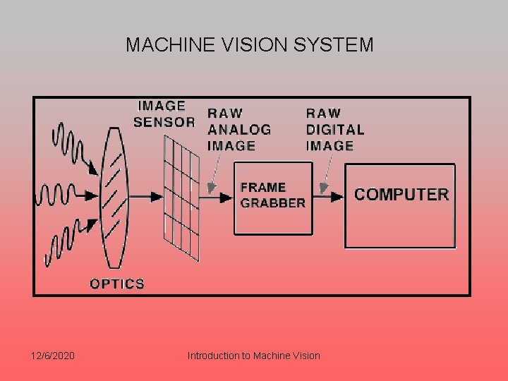
MACHINE VISION SYSTEM 12/6/2020 Introduction to Machine Vision

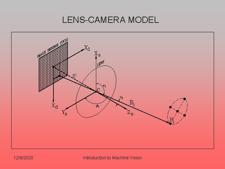
LENS-CAMERA MODEL 12/6/2020 Introduction to Machine Vision

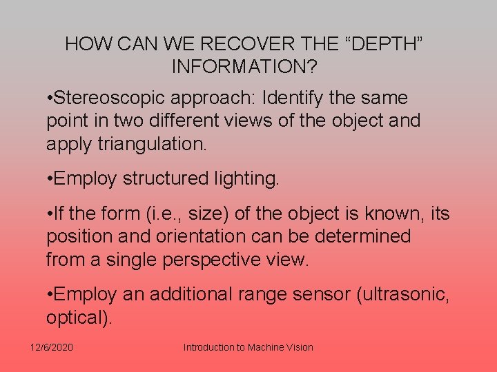
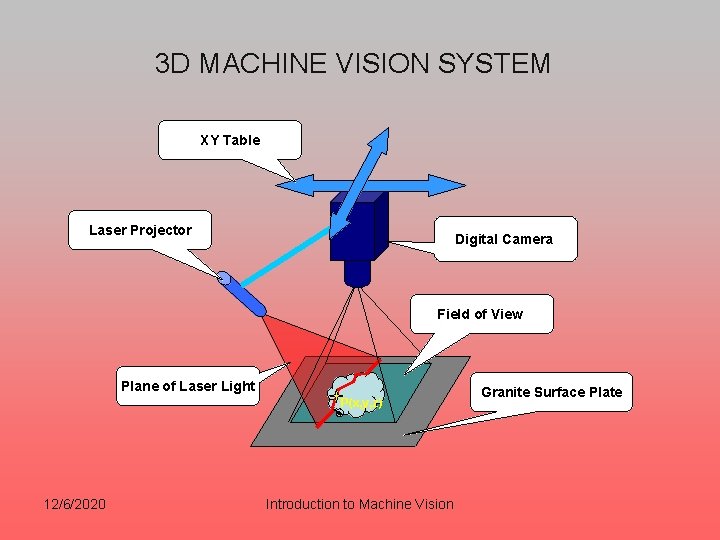
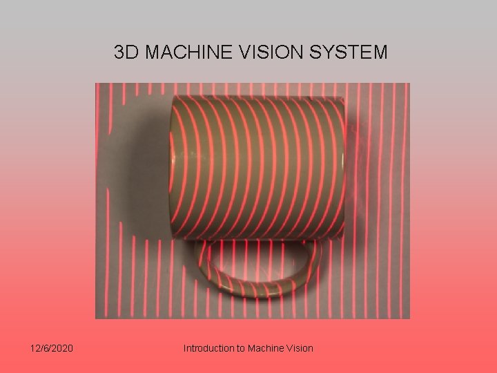
HOW CAN WE RECOVER THE “DEPTH” INFORMATION? • Stereoscopic approach: Identify the same point in two different views of the object and apply triangulation. • Employ structured lighting. • If the form (i. e. , size) of the object is known, its position and orientation can be determined from a single perspective view. • Employ an additional range sensor (ultrasonic, optical). 12/6/2020 Introduction to Machine Vision

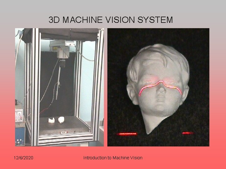
3 D MACHINE VISION SYSTEM XY Table Laser Projector Digital Camera Field of View Plane of Laser Light P(x, y, z) 12/6/2020 Introduction to Machine Vision Granite Surface Plate

3 D MACHINE VISION SYSTEM 12/6/2020 Introduction to Machine Vision

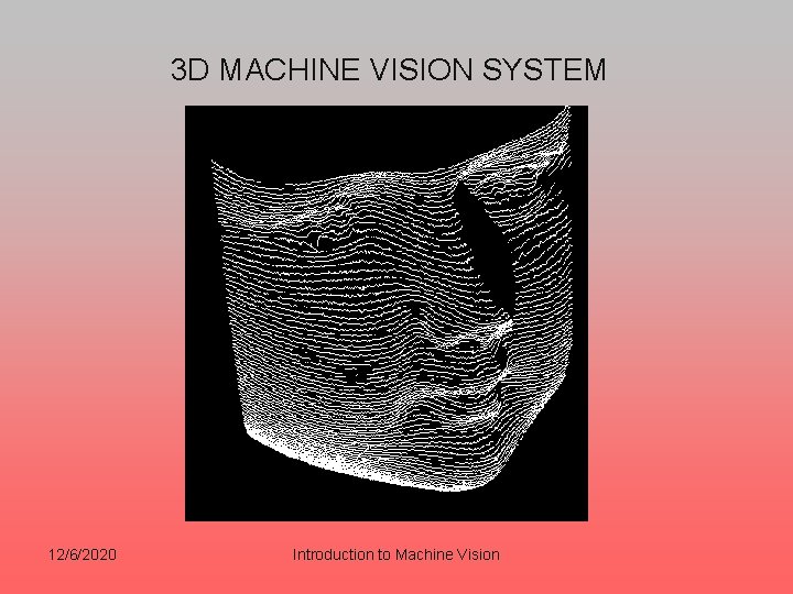
3 D MACHINE VISION SYSTEM 12/6/2020 Introduction to Machine Vision

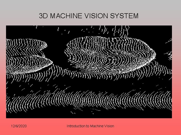
3 D MACHINE VISION SYSTEM 12/6/2020 Introduction to Machine Vision

3 D MACHINE VISION SYSTEM 12/6/2020 Introduction to Machine Vision

2 D MACHINE VISION SYSTEMS • 2 D machine vision deals with image analysis. • The goal of this analysis is to generate a high level description of the input image or scene that can be used (for example) to: • Identify objects in the image (e. g. , character recognition) • Determine the position and orientation of the objects in the image (e. g. , robot assembly) • Inspect the objects in the image (e. g. , PCB inspection) • In all of these examples, the description refers to specific objects or regions in the image. • To generate the description of the image, it is first necessary to segment the image into these regions. 12/6/2020 Introduction to Machine Vision

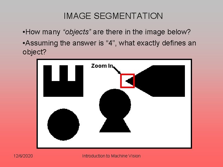
IMAGE SEGMENTATION • How many “objects” are there in the image below? • Assuming the answer is “ 4”, what exactly defines an object? Zoom In 12/6/2020 Introduction to Machine Vision

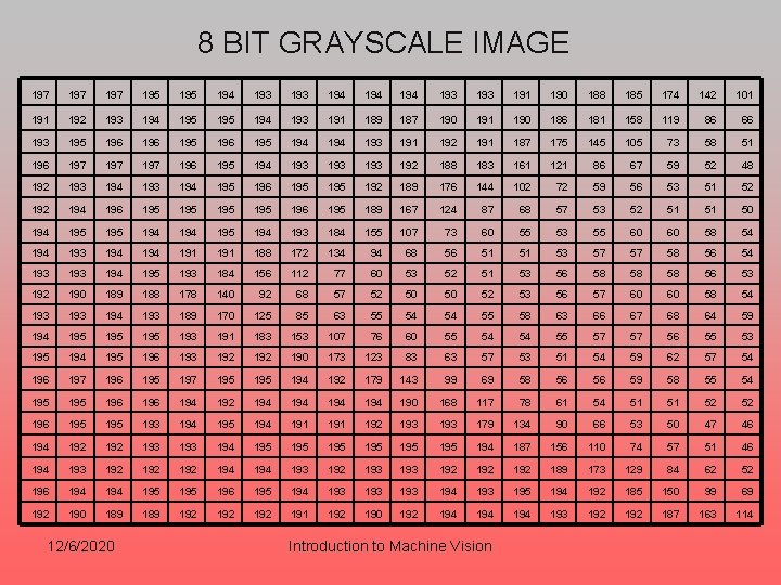
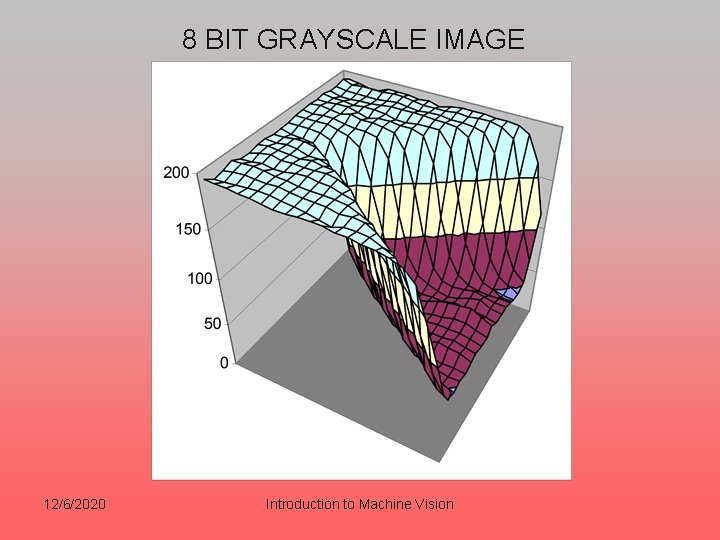
8 BIT GRAYSCALE IMAGE 197 197 195 194 193 194 194 193 191 190 188 185 174 142 101 192 193 194 195 194 193 191 189 187 190 191 190 186 181 158 119 86 66 193 195 196 195 194 193 191 192 191 187 175 145 105 73 58 51 196 197 197 196 195 194 193 193 192 188 183 161 121 86 67 59 52 48 192 193 194 195 196 195 192 189 176 144 102 72 59 56 53 51 52 194 196 195 195 196 195 189 167 124 87 68 57 53 52 51 51 50 194 195 194 193 184 155 107 73 60 55 53 55 60 60 58 54 193 194 191 188 172 134 94 68 56 51 51 53 57 57 58 56 54 193 194 195 193 184 156 112 77 60 53 52 51 53 56 58 58 58 56 53 192 190 189 188 178 140 92 68 57 52 50 50 52 53 56 57 60 60 58 54 193 194 193 189 170 125 85 63 55 54 54 55 58 63 66 67 68 64 59 194 195 195 193 191 183 153 107 76 60 55 54 54 55 57 57 56 55 53 195 194 195 196 193 192 190 173 123 83 63 57 53 51 54 59 62 57 54 196 197 196 195 197 195 194 192 179 143 99 69 58 56 56 59 58 55 54 195 196 194 192 194 194 190 168 117 78 61 54 51 51 52 52 196 195 193 194 195 194 191 192 193 179 134 90 66 53 50 47 46 194 192 193 194 195 195 195 194 187 156 110 74 57 51 46 194 193 192 192 194 193 192 192 189 173 129 84 62 52 196 194 195 196 195 194 193 193 194 193 195 194 192 185 150 99 69 192 190 189 192 192 191 192 190 192 194 194 193 192 187 163 114 12/6/2020 Introduction to Machine Vision

8 BIT GRAYSCALE IMAGE 12/6/2020 Introduction to Machine Vision

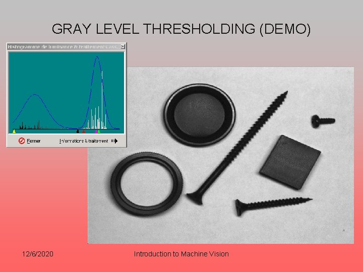
GRAY LEVEL THRESHOLDING • Many images consist of two regions that occupy different gray level ranges. • Such images are characterized by a bimodal image histogram. • An image histogram is a function h defined on the set of gray levels in a given image. • The value h(k) is given by the number of pixels in the image having image intensity k. 12/6/2020 Introduction to Machine Vision

GRAY LEVEL THRESHOLDING (DEMO) 12/6/2020 Introduction to Machine Vision

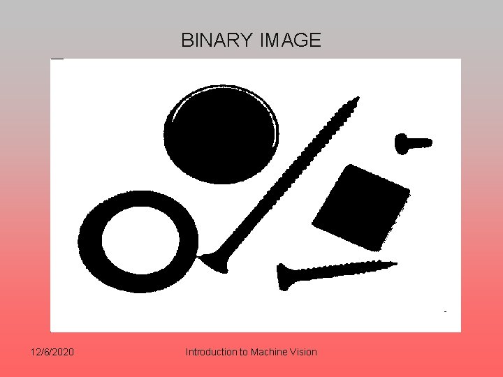
BINARY IMAGE 12/6/2020 Introduction to Machine Vision

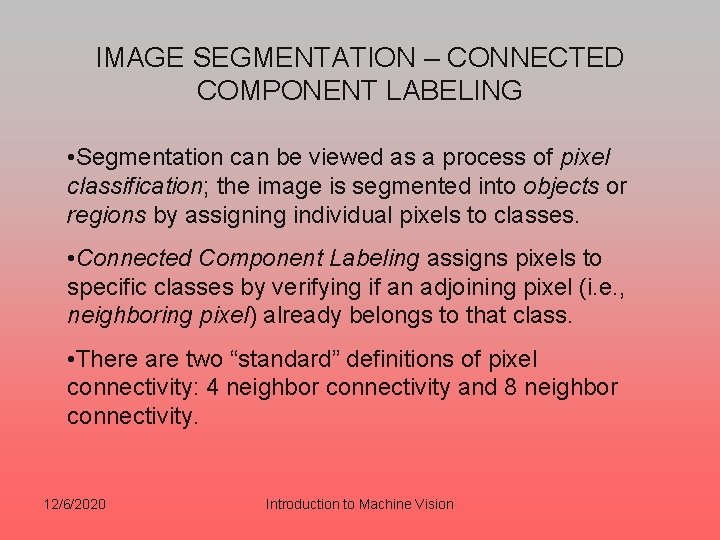
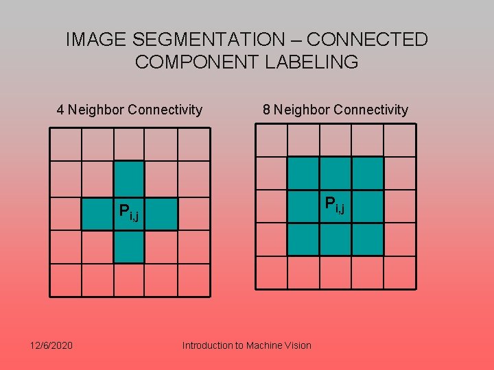
IMAGE SEGMENTATION – CONNECTED COMPONENT LABELING • Segmentation can be viewed as a process of pixel classification; the image is segmented into objects or regions by assigning individual pixels to classes. • Connected Component Labeling assigns pixels to specific classes by verifying if an adjoining pixel (i. e. , neighboring pixel) already belongs to that class. • There are two “standard” definitions of pixel connectivity: 4 neighbor connectivity and 8 neighbor connectivity. 12/6/2020 Introduction to Machine Vision

IMAGE SEGMENTATION – CONNECTED COMPONENT LABELING 4 Neighbor Connectivity 8 Neighbor Connectivity Pi, j 12/6/2020 Introduction to Machine Vision

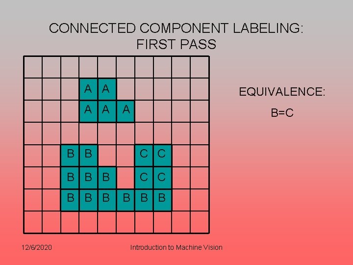
CONNECTED COMPONENT LABELING: FIRST PASS A A 12/6/2020 EQUIVALENCE: A B=C B B C C B B B B Introduction to Machine Vision

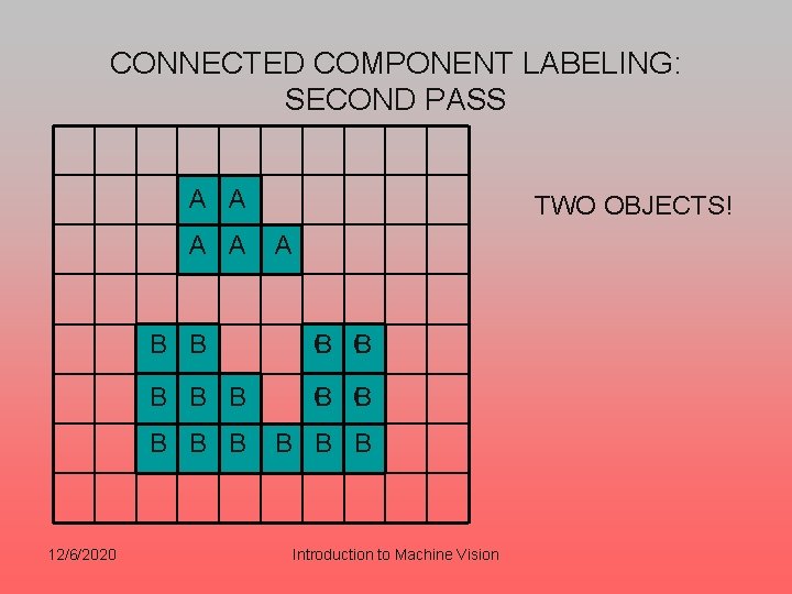
CONNECTED COMPONENT LABELING: SECOND PASS A A 12/6/2020 TWO OBJECTS! A B B C B C B B B B B Introduction to Machine Vision

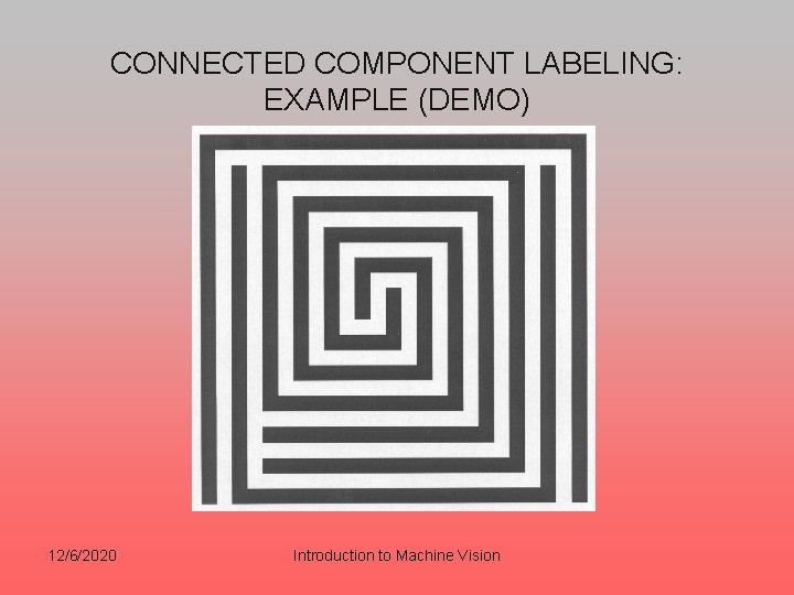
CONNECTED COMPONENT LABELING: EXAMPLE (DEMO) 12/6/2020 Introduction to Machine Vision

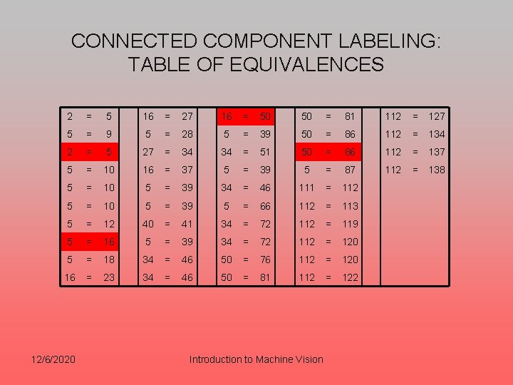
CONNECTED COMPONENT LABELING: TABLE OF EQUIVALENCES 2 = 5 16 = 27 16 = 50 50 = 81 112 = 127 5 = 9 5 = 28 5 = 39 50 = 86 112 = 134 2 = 5 27 = 34 34 = 51 50 = 86 112 = 137 5 = 10 16 = 37 5 = 39 5 = 87 112 = 138 5 = 10 5 = 39 34 = 46 111 = 112 5 = 10 5 = 39 5 = 66 112 = 113 5 = 12 40 = 41 34 = 72 112 = 119 5 = 16 5 = 39 34 = 72 112 = 120 5 = 18 34 = 46 50 = 76 112 = 120 16 = 23 34 = 46 50 = 81 112 = 122 12/6/2020 Introduction to Machine Vision

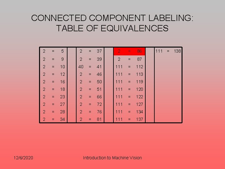
CONNECTED COMPONENT LABELING: TABLE OF EQUIVALENCES 12/6/2020 2 = 5 2 = 37 2 = 86 2 = 9 2 = 39 2 = 87 2 = 10 40 = 41 111 = 112 2 = 46 111 = 113 2 = 16 2 = 50 111 = 119 2 = 18 2 = 51 111 = 120 2 = 23 2 = 66 111 = 122 2 = 27 2 = 72 111 = 127 2 = 28 2 = 76 111 = 134 2 = 81 111 = 137 Introduction to Machine Vision 111 = 138

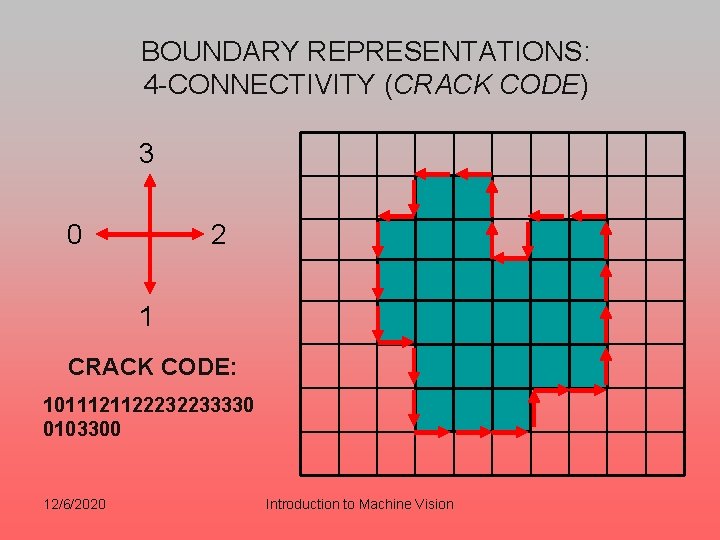
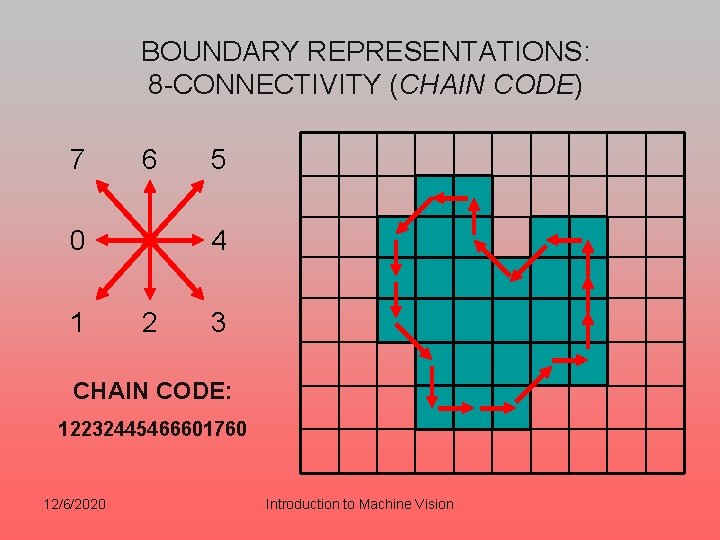
IS THERE A MORE COMPUTATIONALLY EFFICIENT TECHNIQUE FOR SEGMENTING THE OBJECTS IN THE IMAGE? • Contour tracking/border following identify the pixels that fall on the boundaries of the objects, i. e. , pixels that have a neighbor that belongs to the background class or region. • There are two “standard” code definitions used to represent boundaries: code definitions based on 4 connectivity (crack code) and code definitions based on 8 -connectivity (chain code). 12/6/2020 Introduction to Machine Vision

BOUNDARY REPRESENTATIONS: 4 -CONNECTIVITY (CRACK CODE) 3 0 2 1 CRACK CODE: 1011121122232233330 0103300 12/6/2020 Introduction to Machine Vision

BOUNDARY REPRESENTATIONS: 8 -CONNECTIVITY (CHAIN CODE) 7 6 0 1 5 4 2 3 CHAIN CODE: 12232445466601760 12/6/2020 Introduction to Machine Vision

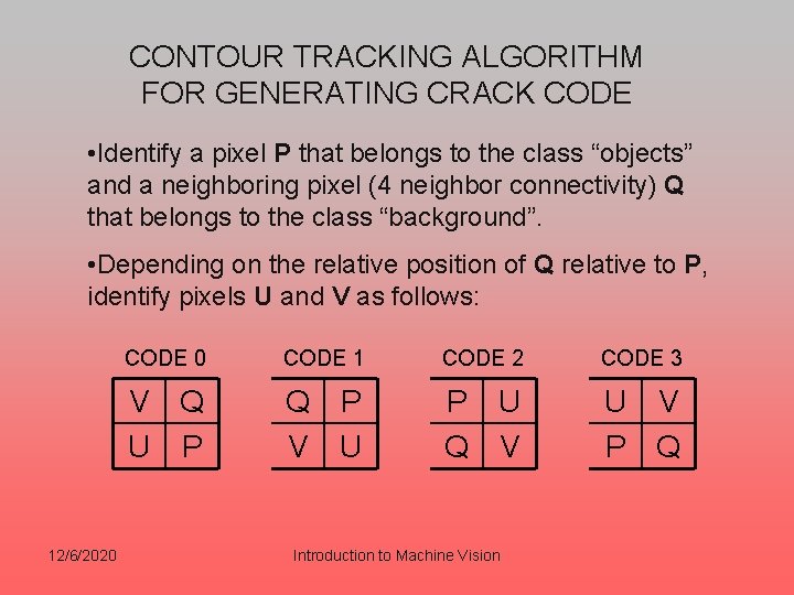
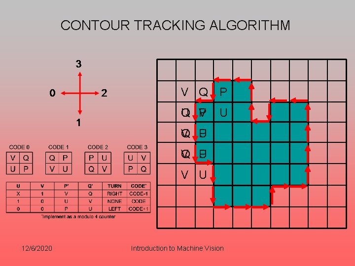
CONTOUR TRACKING ALGORITHM FOR GENERATING CRACK CODE • Identify a pixel P that belongs to the class “objects” and a neighboring pixel (4 neighbor connectivity) Q that belongs to the class “background”. • Depending on the relative position of Q relative to P, identify pixels U and V as follows: 12/6/2020 CODE 1 CODE 2 CODE 3 V Q U P Q P V U P U Q V U V P Q Introduction to Machine Vision

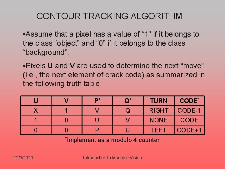
CONTOUR TRACKING ALGORITHM • Assume that a pixel has a value of “ 1” if it belongs to the class “object” and “ 0” if it belongs to the class “background”. • Pixels U and V are used to determine the next “move” (i. e. , the next element of crack code) as summarized in the following truth table: U V P’ Q’ TURN CODE* X 1 V Q RIGHT CODE-1 1 0 U V NONE CODE 0 0 P U LEFT CODE+1 *Implement as a modulo 4 counter 12/6/2020 Introduction to Machine Vision

CONTOUR TRACKING ALGORITHM V Q P U V P Q U V U 12/6/2020 Introduction to Machine Vision

CONTOUR TRACKING ALGORITHM FOR GENERATING CRACK CODE • Software Demo! 12/6/2020 Introduction to Machine Vision

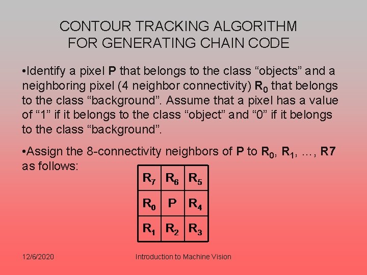
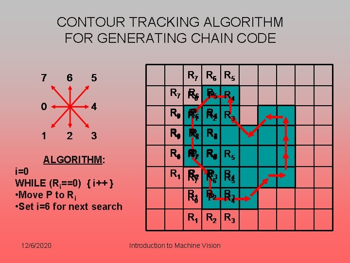
CONTOUR TRACKING ALGORITHM FOR GENERATING CHAIN CODE • Identify a pixel P that belongs to the class “objects” and a neighboring pixel (4 neighbor connectivity) R 0 that belongs to the class “background”. Assume that a pixel has a value of “ 1” if it belongs to the class “object” and “ 0” if it belongs to the class “background”. • Assign the 8 -connectivity neighbors of P to R 0, R 1, …, R 7 as follows: 12/6/2020 Introduction to Machine Vision

CONTOUR TRACKING ALGORITHM FOR GENERATING CHAIN CODE ALGORITHM: i=0 WHILE (Ri==0) { i++ } • Move P to Ri • Set i=6 for next search 12/6/2020 Introduction to Machine Vision

OBJECT RECOGNITION – BLOB ANALYSIS • Once the image has been segmented into classes representing the objects in the image, the next step is to generate a high level description of the various objects. • A comprehensive set of form parameters describing each object or region in an image is useful for object recognition. • Ideally the form parameters should be independent of the object’s position and orientation as well as the distance between the camera and the object (i. e. , scale factor). 12/6/2020 Introduction to Machine Vision

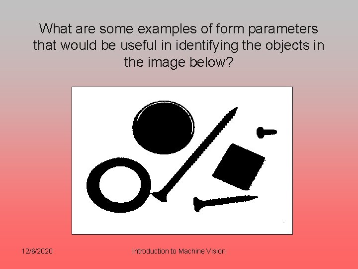
What are some examples of form parameters that would be useful in identifying the objects in the image below? 12/6/2020 Introduction to Machine Vision

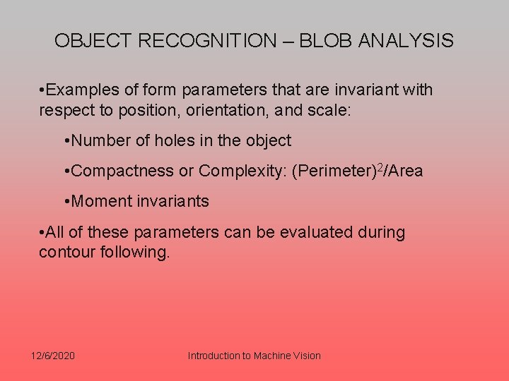
OBJECT RECOGNITION – BLOB ANALYSIS • Examples of form parameters that are invariant with respect to position, orientation, and scale: • Number of holes in the object • Compactness or Complexity: (Perimeter)2/Area • Moment invariants • All of these parameters can be evaluated during contour following. 12/6/2020 Introduction to Machine Vision

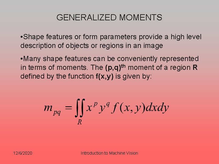
GENERALIZED MOMENTS • Shape features or form parameters provide a high level description of objects or regions in an image • Many shape features can be conveniently represented in terms of moments. The (p, q)th moment of a region R defined by the function f(x, y) is given by: 12/6/2020 Introduction to Machine Vision

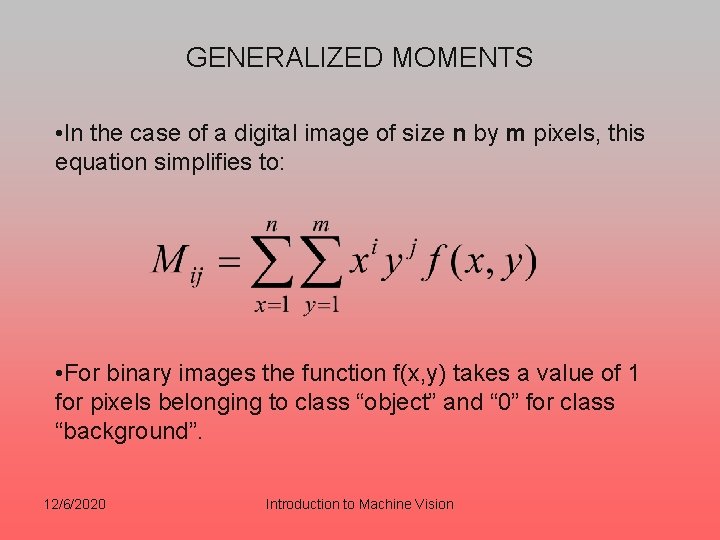
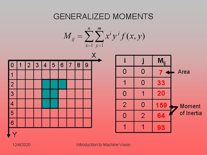
GENERALIZED MOMENTS • In the case of a digital image of size n by m pixels, this equation simplifies to: • For binary images the function f(x, y) takes a value of 1 for pixels belonging to class “object” and “ 0” for class “background”. 12/6/2020 Introduction to Machine Vision

GENERALIZED MOMENTS X i j Mij 1 0 0 Area 2 1 0 3 0 1 7 33 20 4 2 0 5 0 2 159 64 Moment of Inertia 1 1 93 0 1 2 3 4 5 6 7 8 9 6 Y 12/6/2020 Introduction to Machine Vision

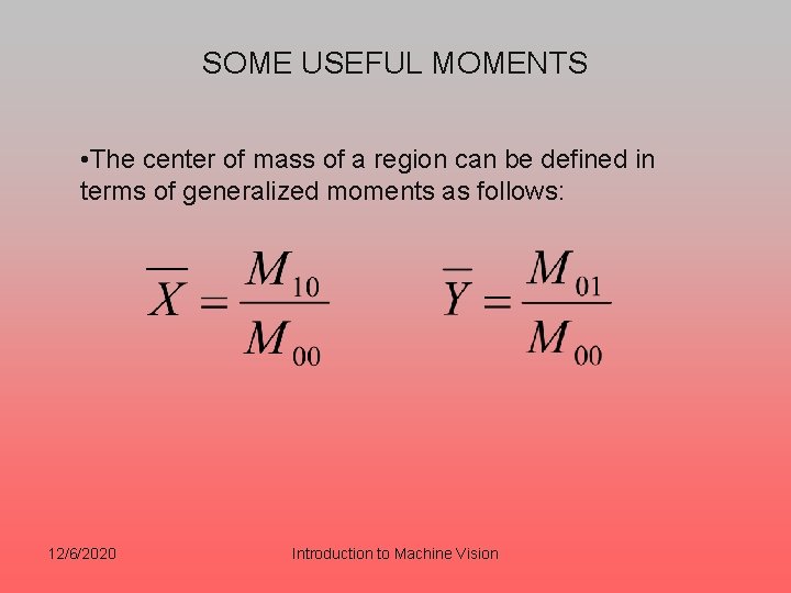
SOME USEFUL MOMENTS • The center of mass of a region can be defined in terms of generalized moments as follows: 12/6/2020 Introduction to Machine Vision

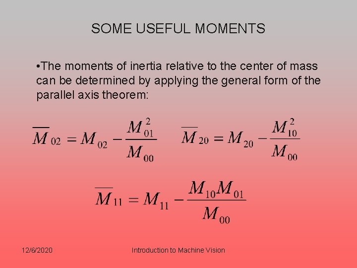
SOME USEFUL MOMENTS • The moments of inertia relative to the center of mass can be determined by applying the general form of the parallel axis theorem: 12/6/2020 Introduction to Machine Vision

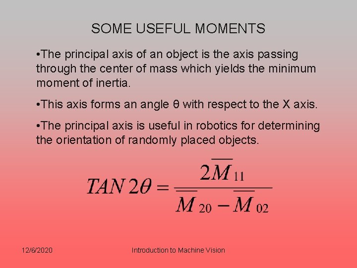
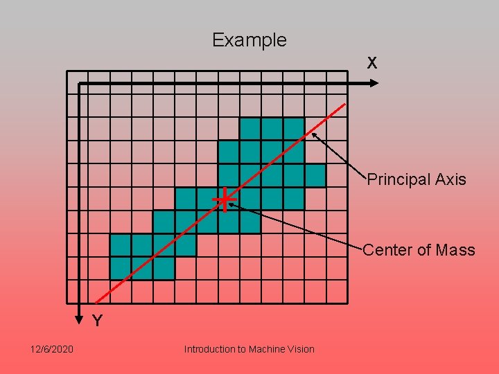
SOME USEFUL MOMENTS • The principal axis of an object is the axis passing through the center of mass which yields the minimum moment of inertia. • This axis forms an angle θ with respect to the X axis. • The principal axis is useful in robotics for determining the orientation of randomly placed objects. 12/6/2020 Introduction to Machine Vision

Example X Principal Axis Center of Mass Y 12/6/2020 Introduction to Machine Vision

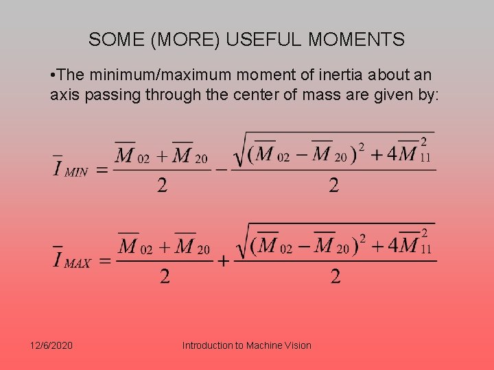
SOME (MORE) USEFUL MOMENTS • The minimum/maximum moment of inertia about an axis passing through the center of mass are given by: 12/6/2020 Introduction to Machine Vision

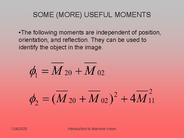
SOME (MORE) USEFUL MOMENTS • The following moments are independent of position, orientation, and reflection. They can be used to identify the object in the image. 12/6/2020 Introduction to Machine Vision

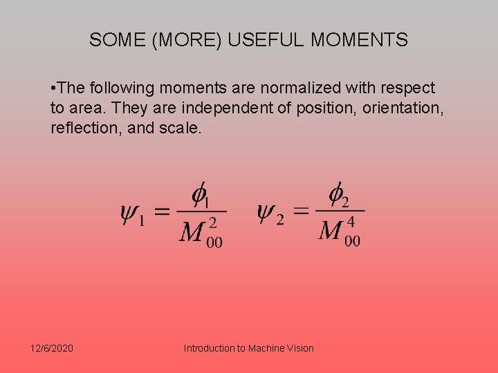
SOME (MORE) USEFUL MOMENTS • The following moments are normalized with respect to area. They are independent of position, orientation, reflection, and scale. 12/6/2020 Introduction to Machine Vision

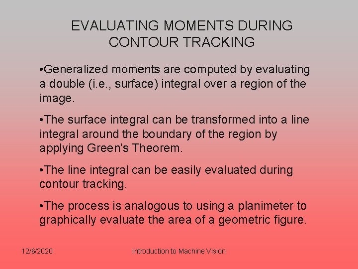
EVALUATING MOMENTS DURING CONTOUR TRACKING • Generalized moments are computed by evaluating a double (i. e. , surface) integral over a region of the image. • The surface integral can be transformed into a line integral around the boundary of the region by applying Green’s Theorem. • The line integral can be easily evaluated during contour tracking. • The process is analogous to using a planimeter to graphically evaluate the area of a geometric figure. 12/6/2020 Introduction to Machine Vision

EVALUATING MOMENTS DIRECTLY FROM CRACK CODE DURING CONTOUR TRACKING { switch ( code [i] ) { case 0: m 00 = m 00 - y; m 01 = m 01 - sum_y; m 02 = m 02 - sum_y 2; x = x - 1; sum_x = sum_x - x; sum_x 2 = sum_x 2 - x*x; m 11 = m 11 - (x*sum_y); break; 12/6/2020 case 1: sum_y = sum_y + y; sum_y 2 = sum_y 2 + y*y; y = y + 1; m 10 = m 10 - sum_x; m 20 = m 20 - sum_x 2; break; Introduction to Machine Vision

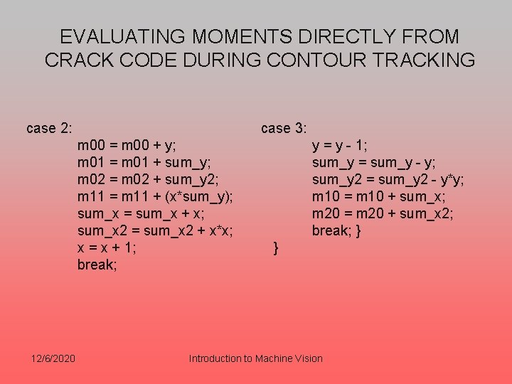
EVALUATING MOMENTS DIRECTLY FROM CRACK CODE DURING CONTOUR TRACKING case 2: case 3: m 00 = m 00 + y; m 01 = m 01 + sum_y; m 02 = m 02 + sum_y 2; m 11 = m 11 + (x*sum_y); sum_x = sum_x + x; sum_x 2 = sum_x 2 + x*x; x = x + 1; break; y = y - 1; sum_y = sum_y - y; sum_y 2 = sum_y 2 - y*y; m 10 = m 10 + sum_x; m 20 = m 20 + sum_x 2; break; } } 12/6/2020 Introduction to Machine Vision

QUESTIONS ? 12/6/2020 Introduction to Machine Vision