Mad Max Experiment Algorithm to Place Discs Mad

Mad. Max Experiment: Algorithm to Place Discs Mad. Max Mini Workshop MPP C. Moore November 21, 2016 Slide 1 C. Moore / MPP

Outline • Resonator Control: Problem Background • Obtaining S 11 (Reflection) Frequency Response ▫ Measurement ▫ Simulation - Vector Network Analysis - ADS/Qucs • Signal Processing ▫ A direct comparison ▫ Problems with Experiment and Model ▫ Signal Flow Diagram • Fitting Algorithm ▫ Starting Point: A Naive Genetic Algorithm for Best Fit ▫ Control Strategies • Initial Results • Refined Model • Ongoing Work Slide 2 C. Moore / MPP

Resonator Control Problem Background Slide 3 C. Moore / MPP

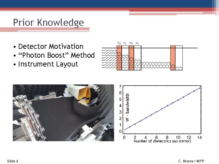
Prior Knowledge • Detector Motivation • “Photon Boost” Method • Instrument Layout Slide 4 C. Moore / MPP

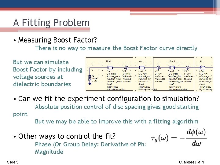
A Fitting Problem • Measuring Boost Factor? There is no way to measure the Boost Factor curve directly But we can simulate Boost Factor by including voltage sources at dielectric boundaries • Can we fit the experiment configuration to simulation? Absolute position control of disc spacing gives good starting point But we may be able to improve this with a fitting algorithm • Other ways to control the fit? Phase (Or Group Delay: Derivative of Phase) Magnitude Slide 5 C. Moore / MPP

Resonator Control Obtaining S 11 (Reflection) Frequency Response Slide 6 C. Moore / MPP

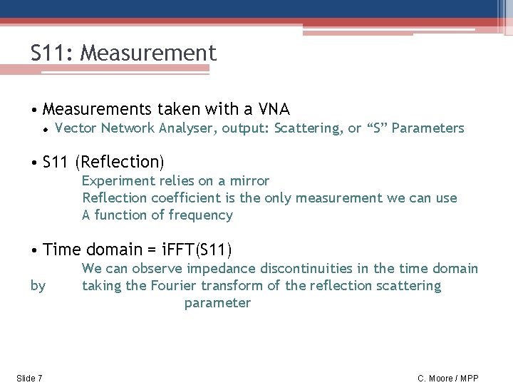
S 11: Measurement • Measurements taken with a VNA Vector Network Analyser, output: Scattering, or “S” Parameters • S 11 (Reflection) Experiment relies on a mirror Reflection coefficient is the only measurement we can use A function of frequency • Time domain = i. FFT(S 11) by Slide 7 We can observe impedance discontinuities in the time domain taking the Fourier transform of the reflection scattering parameter C. Moore / MPP

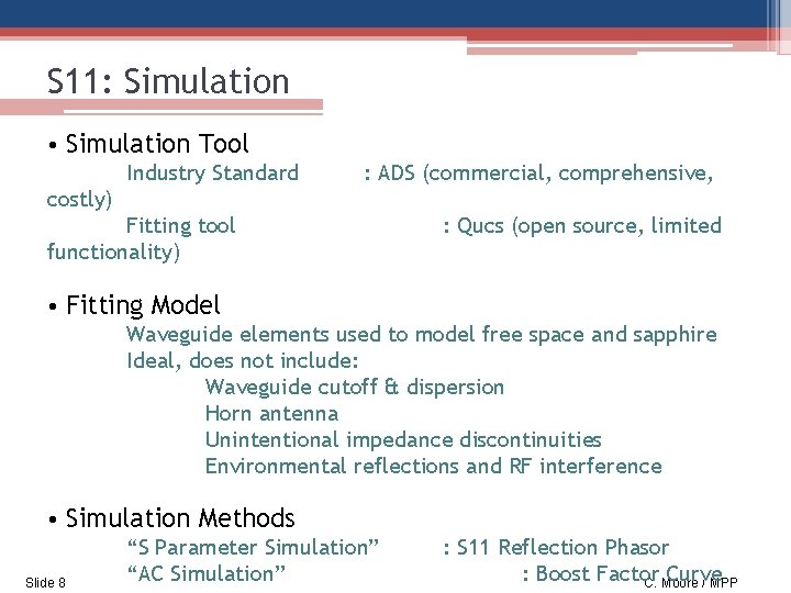
S 11: Simulation • Simulation Tool Industry Standard : ADS (commercial, comprehensive, costly) Fitting tool functionality) : Qucs (open source, limited • Fitting Model Waveguide elements used to model free space and sapphire Ideal, does not include: Waveguide cutoff & dispersion Horn antenna Unintentional impedance discontinuities Environmental reflections and RF interference • Simulation Methods Slide 8 “S Parameter Simulation” “AC Simulation” : S 11 Reflection Phasor : Boost Factor Curve C. Moore / MPP

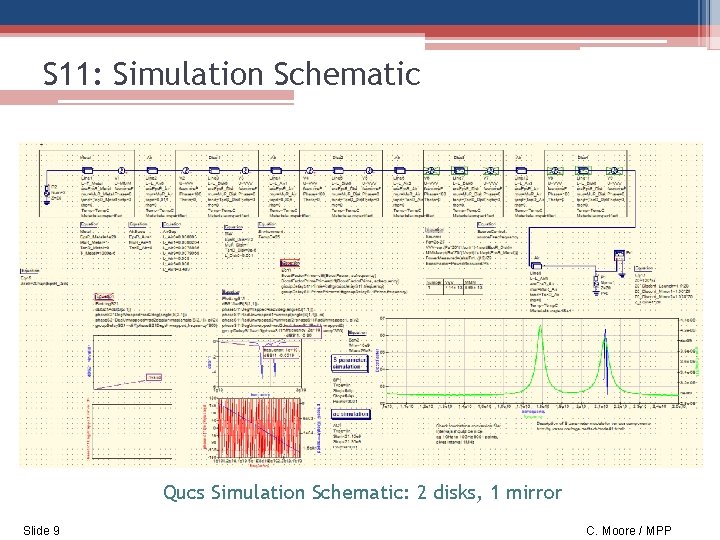
S 11: Simulation Schematic Qucs Simulation Schematic: 2 disks, 1 mirror Slide 9 C. Moore / MPP

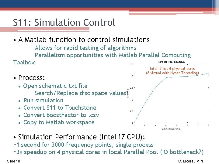
S 11: Simulation Control • A Matlab function to control simulations Allows for rapid testing of algorithms Parallelism opportunities with Matlab Parallel Computing Toolbox • Process: Intel i 7 has 4 physical cores (8 virtual with Hyper-Threading) Open schematic txt file Search/Replace disc space values Run simulation Convert S 11 to Touchstone Convert Boost. Factor to. csv Copy to Matlab workspace • Simulation Performance (Intel i 7 CPU): ~1 second for 3000 frequency points, single process ~3 x speedup on 4 physical cores in local Parallel Pool (IO bottleneck? ) Slide 10 C. Moore / MPP

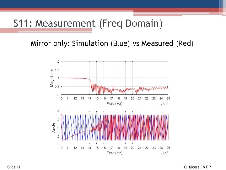
S 11: Measurement (Freq Domain) Mirror only: Simulation (Blue) vs Measured (Red) Slide 11 C. Moore / MPP

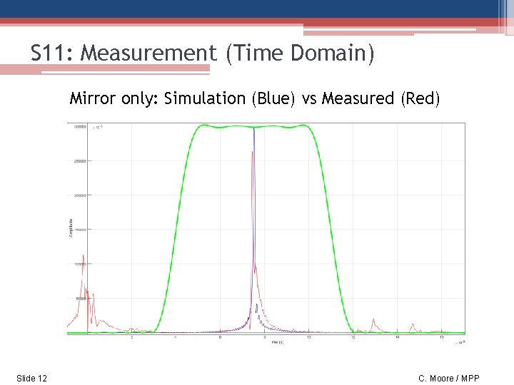
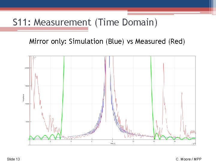
S 11: Measurement (Time Domain) Mirror only: Simulation (Blue) vs Measured (Red) Slide 12 C. Moore / MPP

S 11: Measurement (Time Domain) Mirror only: Simulation (Blue) vs Measured (Red) Slide 13 C. Moore / MPP

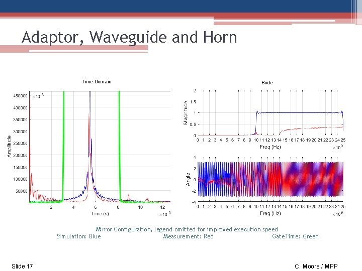
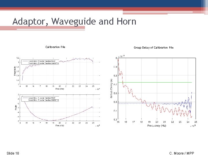
Adaptor, Waveguide and Horn • Some characterstics are difficult to simulate Waveguide Cutoff & Dispersion Capacitive effects Horn effectivity (frequency dependant) & sidelobe loss • Can be calibrated out of measurement Mirror should have a very narrow time impulse response Determine transfer function between gated mirror and simulation Becomes the calibration file, removed from all measurements Requires calibration process and signal processing Slide 14 C. Moore / MPP

Resonator Control Signal Processing Slide 15 C. Moore / MPP

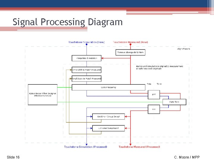
Signal Processing Diagram Slide 16 C. Moore / MPP

Adaptor, Waveguide and Horn Time Domain Bode Mirror Configuration, legend omitted for improved execution speed Simulation: Blue Measurement: Red Gate. Time: Green Slide 17 C. Moore / MPP

Adaptor, Waveguide and Horn Calibration File Slide 18 Group Delay of Calibration File C. Moore / MPP

Installing Discs • 8 mm Configuration, Manually Tuned Experiment: Perform calibration Install a disc, fit to simulation by comparing group delay Repeat, until 4 discs installed Simulation: Separate simulation required for each step Original manual process performed in Lab. View, but replicated here with Matlab Limitations in network analyser (computation and display) More flexibility in signal processing in Matlab Better adjustment of Kaiser Bessel window parameters Slide 19 C. Moore / MPP

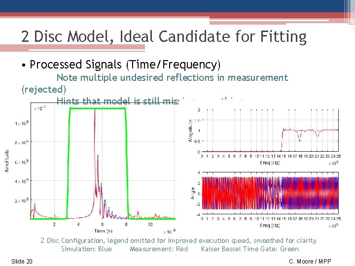
2 Disc Model, Ideal Candidate for Fitting • Processed Signals (Time/Frequency) Note multiple undesired reflections in measurement (rejected) Hints that model is still missing something 2 Disc Configuration, legend omitted for improved execution speed, smoothed for clarity Simulation: Blue Measurement: Red Kaiser Bessel Time Gate: Green Slide 20 C. Moore / MPP

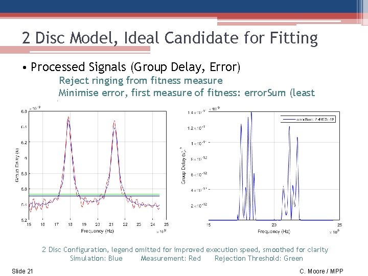
2 Disc Model, Ideal Candidate for Fitting • Processed Signals (Group Delay, Error) Reject ringing from fitness measure Minimise error, first measure of fitness: error. Sum (least squares) 2 Disc Configuration, legend omitted for improved execution speed, smoothed for clarity Simulation: Blue Measurement: Red Rejection Threshold: Green Slide 21 C. Moore / MPP

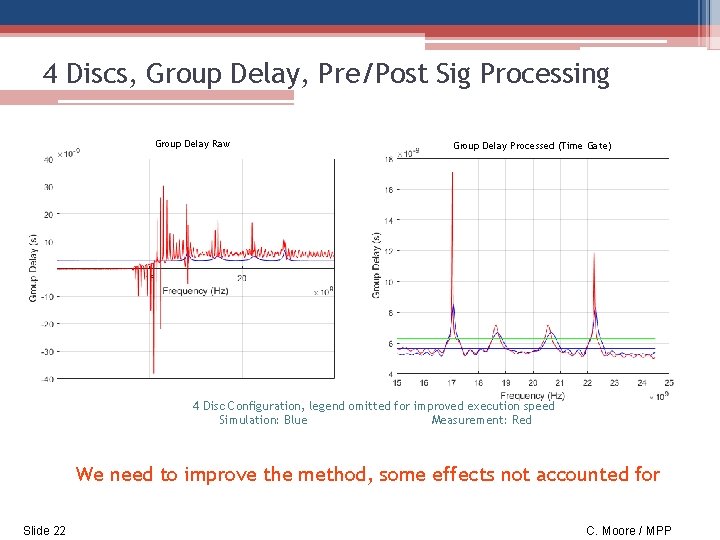
4 Discs, Group Delay, Pre/Post Sig Processing Group Delay Raw Group Delay Processed (Time Gate) 4 Disc Configuration, legend omitted for improved execution speed Simulation: Blue Measurement: Red We need to improve the method, some effects not accounted for Slide 22 C. Moore / MPP

Resonator Control Fitting Algorithm Slide 23 C. Moore / MPP

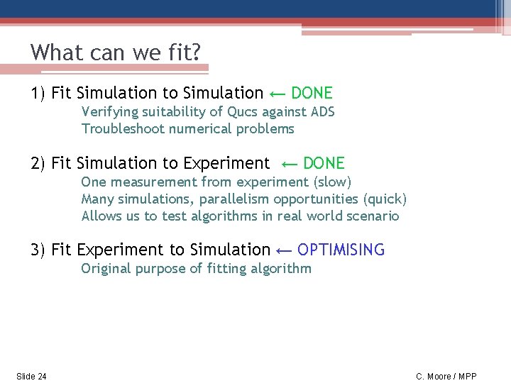
What can we fit? 1) Fit Simulation to Simulation ← DONE Verifying suitability of Qucs against ADS Troubleshoot numerical problems 2) Fit Simulation to Experiment ← DONE One measurement from experiment (slow) Many simulations, parallelism opportunities (quick) Allows us to test algorithms in real world scenario 3) Fit Experiment to Simulation ← OPTIMISING Original purpose of fitting algorithm Slide 24 C. Moore / MPP

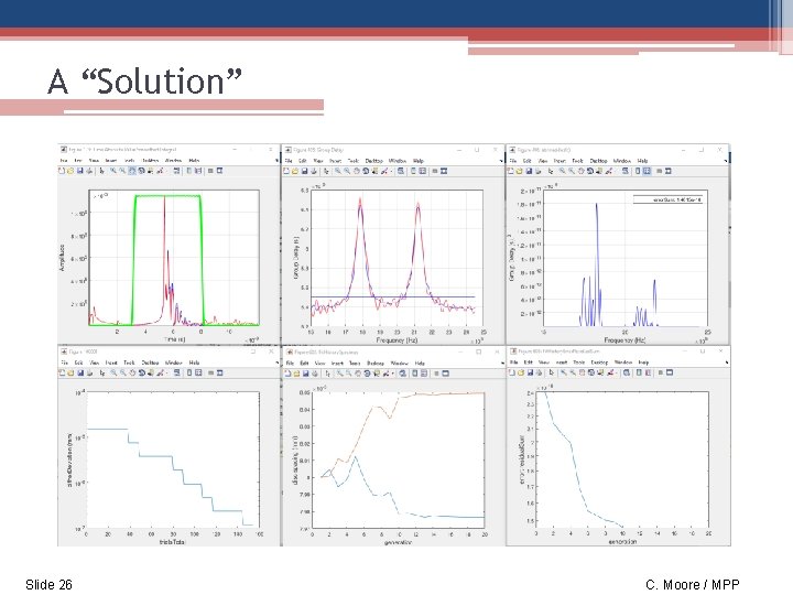
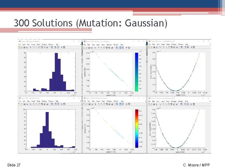
First Algorithm • The System 2 variables (space 1, space 2) 1 fitness measure (Sum of Square Residuals) • Naive Approach Random dither on spacings, close in on the optimal solution Evolutionary/Genetic? Uniform/Normal distribution? • Most Promising Try a configuration based on a wide uniform distribution If improved residual, use this configuration After failing to improve the residual, reduce the random variation Repeat until termination criteria reached (residuals/variation) Now we have one “Solution” Slide 25 C. Moore / MPP

A “Solution” Slide 26 C. Moore / MPP

300 Solutions (Mutation: Gaussian) Slide 27 C. Moore / MPP

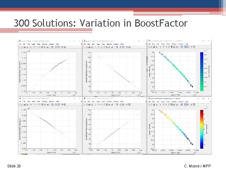
300 Solutions: Variation in Boost. Factor Slide 28 C. Moore / MPP

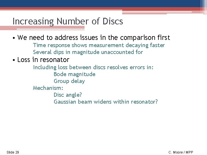
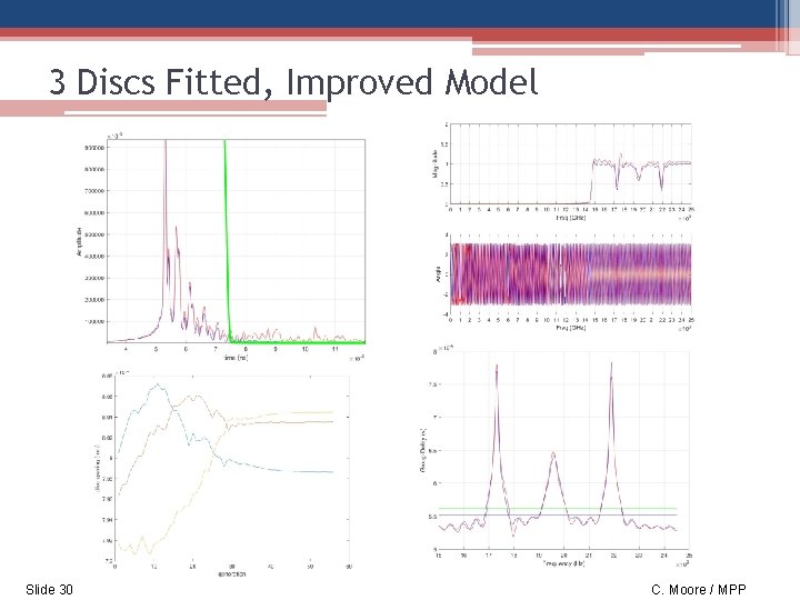
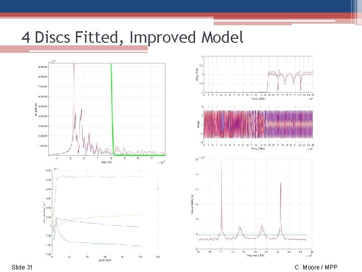
Increasing Number of Discs • We need to address issues in the comparison first Time response shows measurement decaying faster Several dips in magnitude unaccounted for • Loss in resonator Including loss between discs resolves errors in: Bode magnitude Group delay Mechanism: Disc angle? Gaussian beam widens within resonator? Slide 29 C. Moore / MPP

3 Discs Fitted, Improved Model Slide 30 C. Moore / MPP

4 Discs Fitted, Improved Model Slide 31 C. Moore / MPP

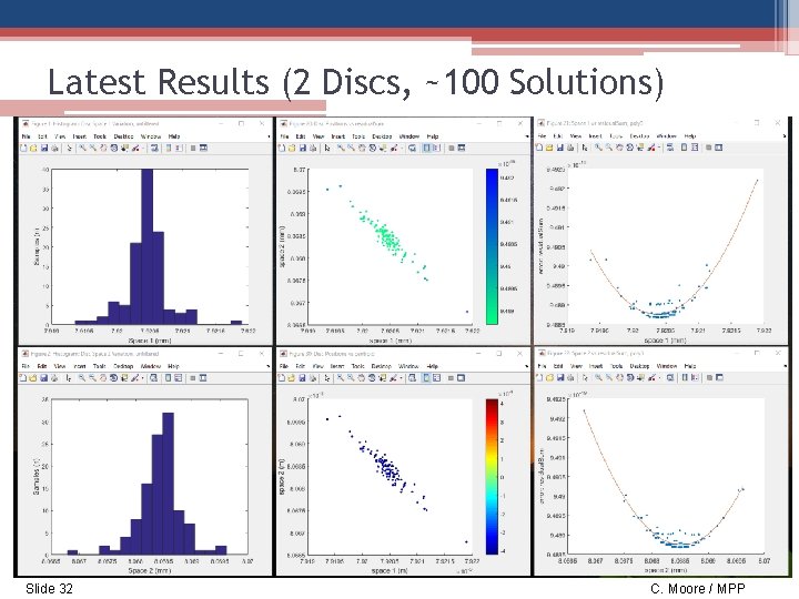
Latest Results (2 Discs, ~100 Solutions) Slide 32 C. Moore / MPP

Latest Results (3 Disc, one “Solution”) Slide 33 C. Moore / MPP

Findings & Further Work • Findings Improved model Group delay peak “sharpness” results from loss between discs Evolutionary/Genetic algorithm fits to better than: +/- 1 um for low disc. N Boost factor peak variation with fit quality • Further Work Cleaner measurement & more accurate model Understanding loss Reducing time to fit instrument to model Currently one solution ~30 min Scaling with number of discs (time to fit, repeatability) Fitting the instrument to arbitrary shapes Thank you for listening Slide 34 C. Moore / MPP