Machine learning for Dynamic Social Network Analysis Applications

Machine learning for Dynamic Social Network Analysis Applications: Control Manuel Gomez Rodriguez Max Planck Institute for Software Systems IJCAI TUTORIAL, AUGUST 2017

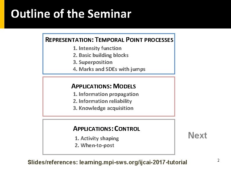
Outline of the Seminar REPRESENTATION: TEMPORAL POINT PROCESSES 1. Intensity function 2. Basic building blocks 3. Superposition 4. Marks and SDEs with jumps APPLICATIONS: MODELS 1. Information propagation 2. Information reliability 3. Knowledge acquisition APPLICATIONS: CONTROL 1. Activity shaping 2. When-to-post Slides/references: learning. mpi-sws. org/ijcai-2017 -tutorial Next 2

Applications: Control 1. Activity shaping 2. When-to-post 3

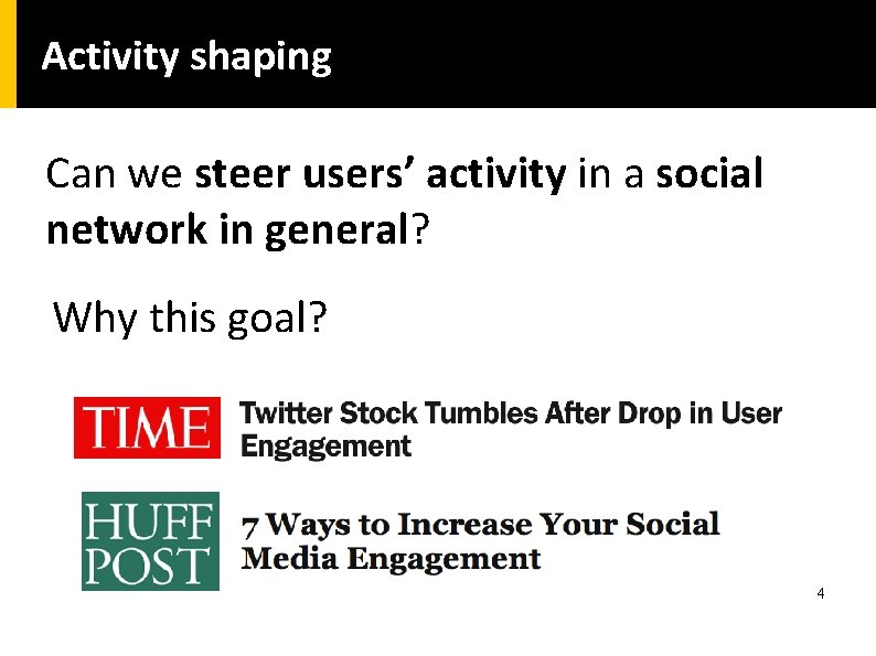
Activity shaping Can we steer users’ activity in a social network in general? Why this goal? 4

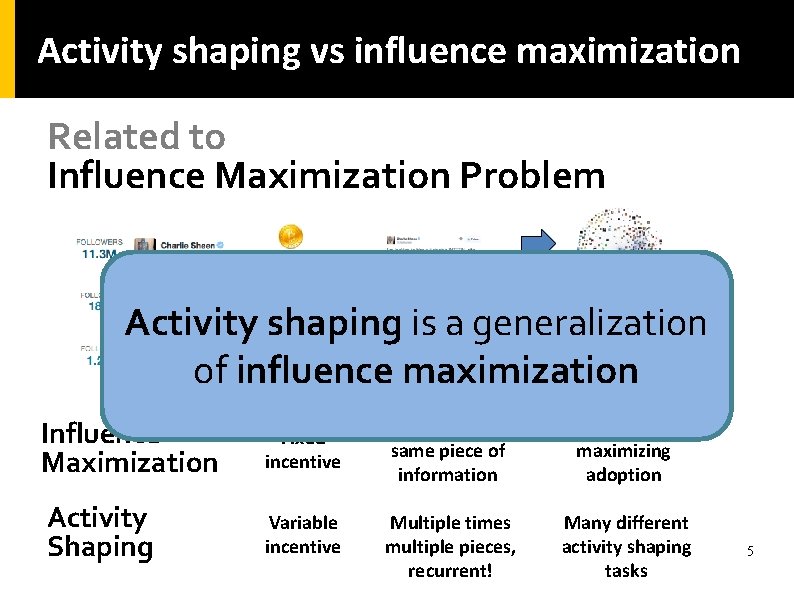
Activity shaping vs influence maximization Related to Influence Maximization Problem Activity shaping is a generalization of influence maximization Influence Maximization Fixed incentive Activity Shaping Variable incentive One time the same piece of information It is only about maximizing adoption Multiple times multiple pieces, recurrent! Many different activity shaping tasks 5

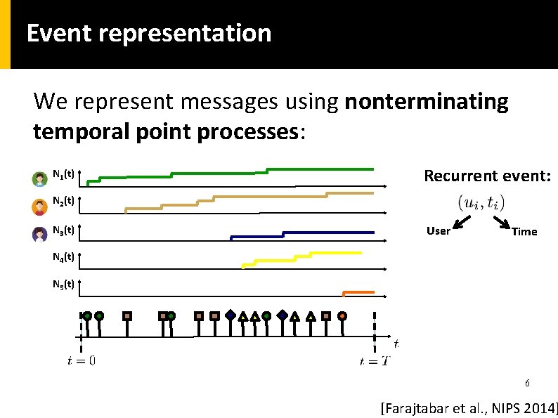
Event representation We represent messages using nonterminating temporal point processes: N 1(t) Recurrent event: N 2(t) N 3(t) User Time N 4(t) N 5(t) 6 [Farajtabar et al. , NIPS 2014]

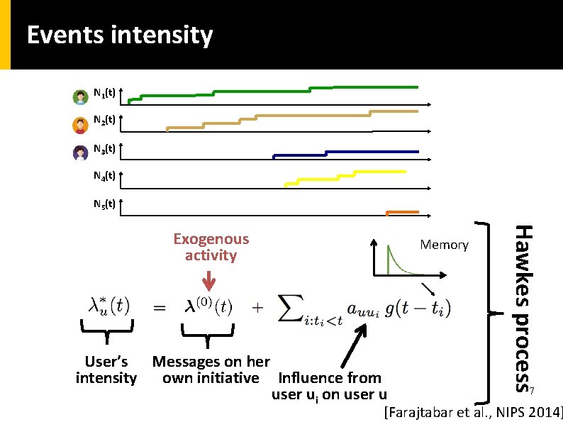
Events intensity N 1(t) N 2(t) N 3(t) N 4(t) N 5(t) Memory User’s Messages on her intensity own initiative Influence from user ui on user u Hawkes process Exogenous activity 7 [Farajtabar et al. , NIPS 2014]

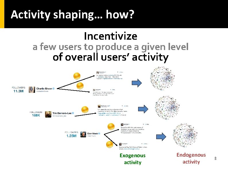
Activity shaping… how? Incentivize a few users to produce a given level of overall users’ activity Exogenous activity Endogenous activity 8

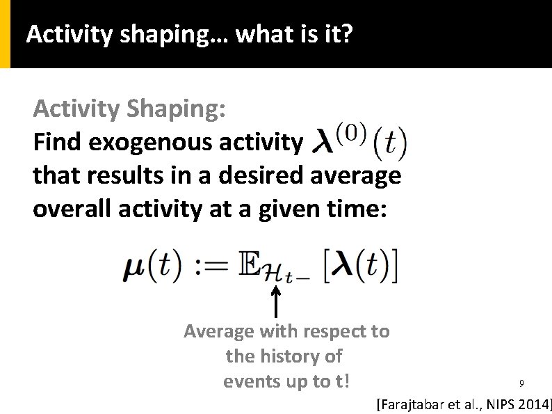
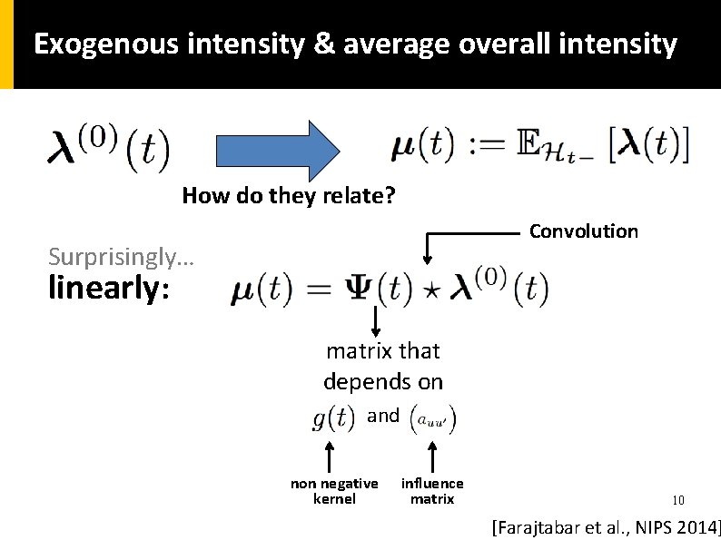
Activity shaping… what is it? Activity Shaping: Find exogenous activity that results in a desired average overall activity at a given time: Average with respect to the history of events up to t! 9 [Farajtabar et al. , NIPS 2014]

Exogenous intensity & average overall intensity How do they relate? Convolution Surprisingly… linearly: matrix that depends on and non negative kernel influence matrix 10 [Farajtabar et al. , NIPS 2014]

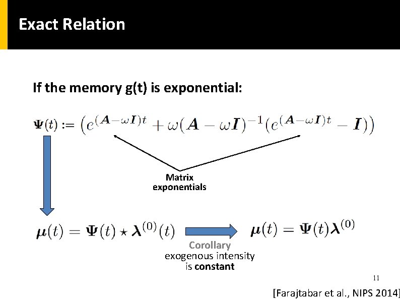
Exact Relation If the memory g(t) is exponential: Matrix exponentials Corollary exogenous intensity is constant 11 [Farajtabar et al. , NIPS 2014]

Does it really work in practice? 12 [Farajtabar et al. , NIPS 2014]

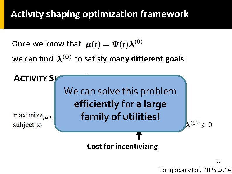
Activity shaping optimization framework Once we know that we can find to satisfy many different goals: ACTIVITY SHAPING PROBLEM We can solve this problem Utility (Goal) Budget efficiently for a large family of utilities! Cost for incentivizing 13 [Farajtabar et al. , NIPS 2014]

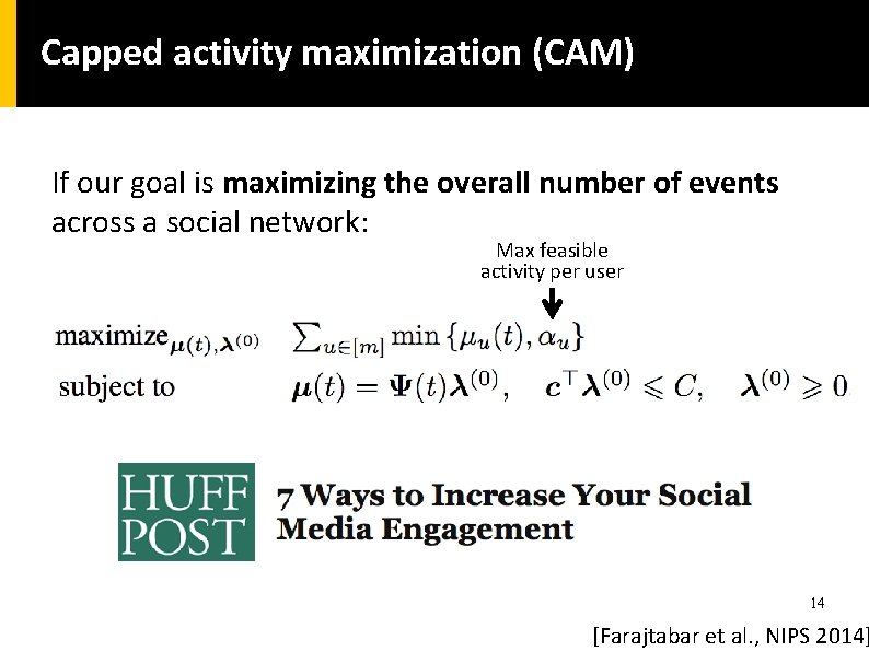
Capped activity maximization (CAM) If our goal is maximizing the overall number of events across a social network: Max feasible activity per user 14 [Farajtabar et al. , NIPS 2014]

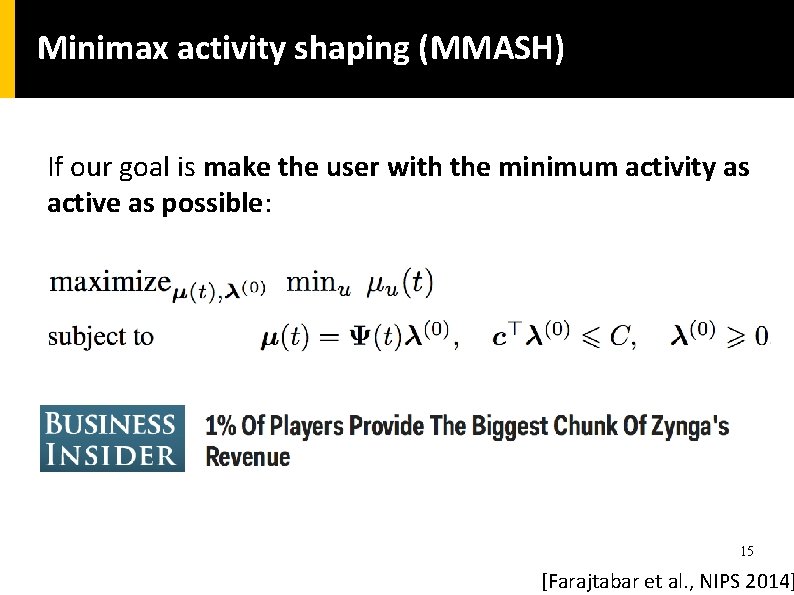
Minimax activity shaping (MMASH) If our goal is make the user with the minimum activity as active as possible: 15 [Farajtabar et al. , NIPS 2014]

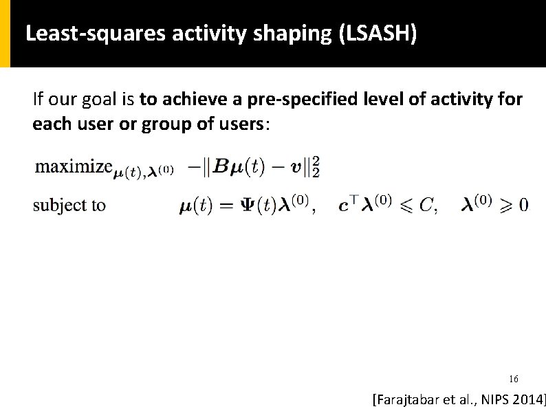
Least-squares activity shaping (LSASH) If our goal is to achieve a pre-specified level of activity for each user or group of users: 16 [Farajtabar et al. , NIPS 2014]

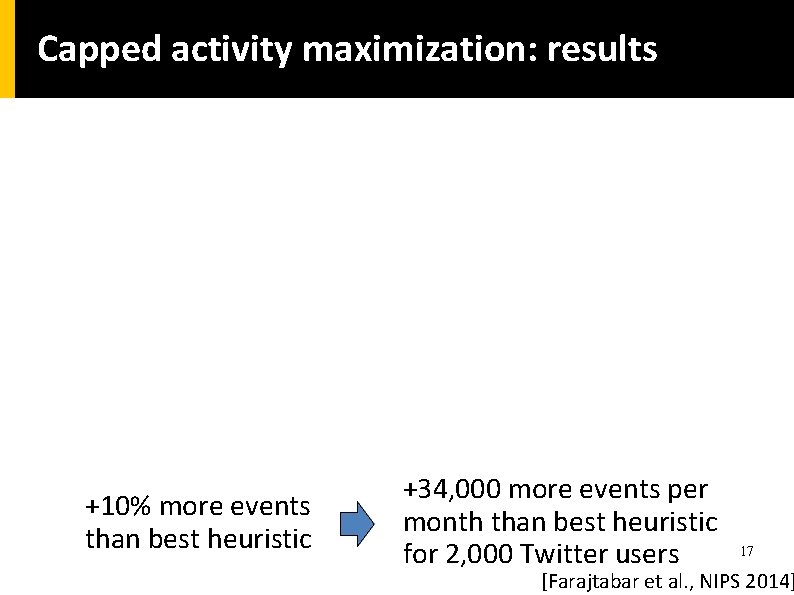
Capped activity maximization: results +10% more events than best heuristic +34, 000 more events per month than best heuristic for 2, 000 Twitter users 17 [Farajtabar et al. , NIPS 2014]

Applications: Control 1. Activity shaping 2. When-to-post 18

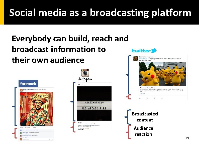
Social media as a broadcasting platform Everybody can build, reach and broadcast information to their own audience Broadcasted content Audience reaction 19

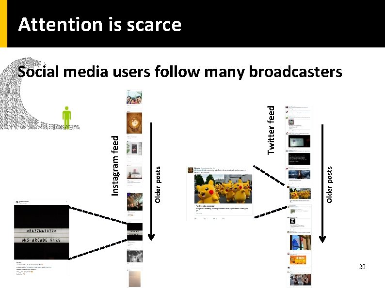
Attention is scarce Older posts Twitter feed Older posts Instagram feed Social media users follow many broadcasters 20

What are the best times to post? Can we design an algorithm that tell us when to post to achieve high visibility? 21

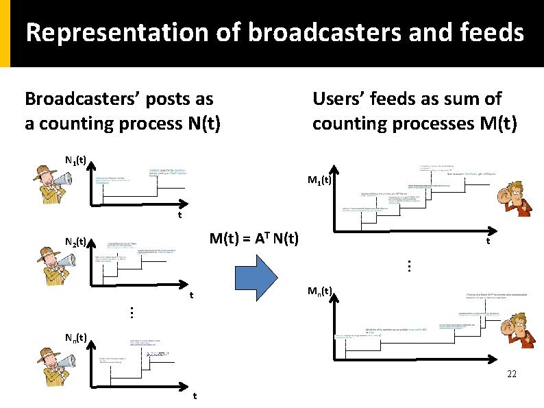
Representation of broadcasters and feeds Broadcasters’ posts as a counting process N(t) Users’ feeds as sum of counting processes M(t) N 1(t) M 1(t) t M(t) = AT N(t) N 2(t) t … Mn(t) t … Nn(t) 22 t

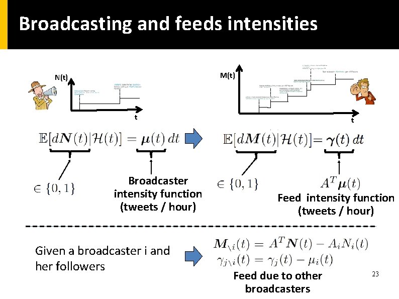
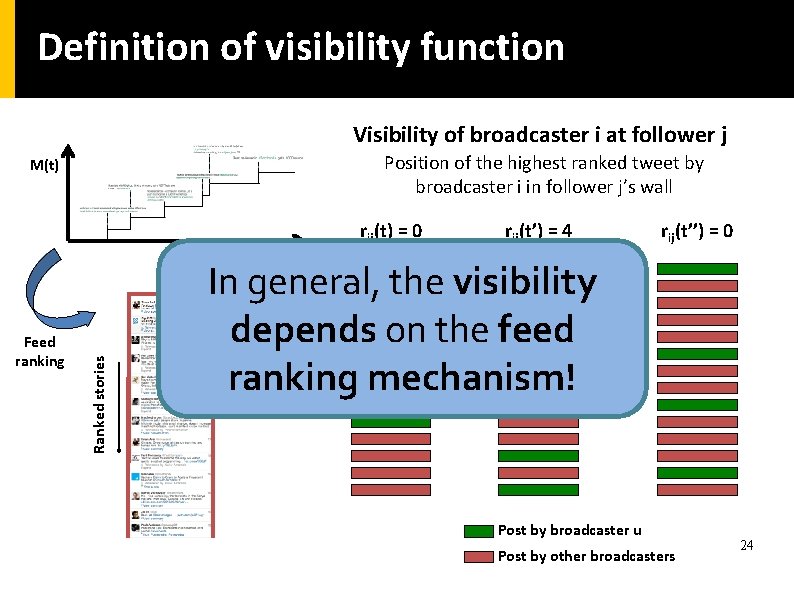
Broadcasting and feeds intensities M(t) N(t) t Broadcaster intensity function (tweets / hour) Given a broadcaster i and her followers t Feed intensity function (tweets / hour) Feed due to other broadcasters 23

Definition of visibility function Visibility of broadcaster i at follower j Position of the highest ranked tweet by broadcaster i in follower j’s wall M(t) rij(t) = 0 In general, the visibility depends on the feed …. ranking mechanism! Older tweets Feed ranking Ranked stories t rij(t’) = 4 rij(t’’) = 0 . Post by broadcaster u Post by other broadcasters 24

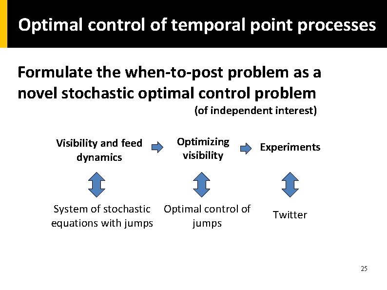
Optimal control of temporal point processes Formulate the when-to-post problem as a novel stochastic optimal control problem (of independent interest) Visibility and feed dynamics Optimizing visibility System of stochastic Optimal control of equations with jumps Experiments Twitter 25

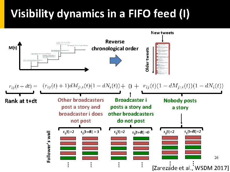
Visibility dynamics in a FIFO feed (I) Reverse chronological order M(t) Older tweets New tweets Other broadcasters Broadcaster i post a story and posts a story and broadcaster i does other broadcasters not post do not post rij(t)=2 rij(t+dt) = 3 rij(t)=2 rij(t+dt) =0 Nobody posts a story rij(t)=2 rij(t+dt)=2 26 … … … Follower’s wall Rank at t+dt [Zarezade et al. , WSDM 2017]

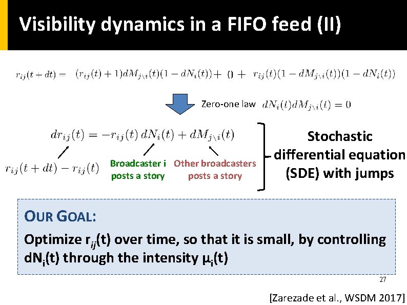
Visibility dynamics in a FIFO feed (II) Zero-one law Broadcaster i Other broadcasters posts a story Stochastic differential equation (SDE) with jumps OUR GOAL: Optimize rij(t) over time, so that it is small, by controlling d. Ni(t) through the intensity μi(t) 27 [Zarezade et al. , WSDM 2017]

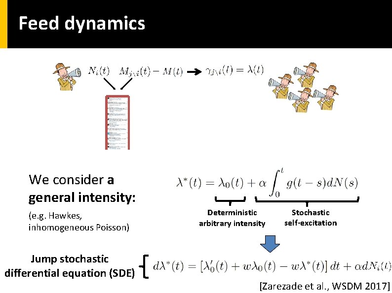
Feed dynamics We consider a general intensity: (e. g. Hawkes, inhomogeneous Poisson) Jump stochastic differential equation (SDE) Deterministic arbitrary intensity Stochastic self-excitation 28 [Zarezade et al. , WSDM 2017]

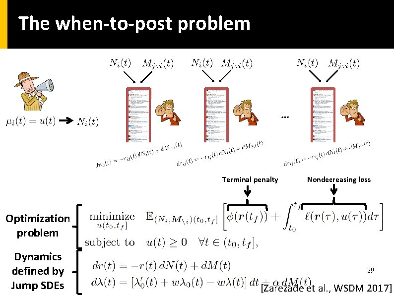
The when-to-post problem … Terminal penalty Nondecreasing loss Optimization problem Dynamics defined by Jump SDEs 29 [Zarezade et al. , WSDM 2017]

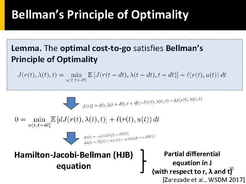
Bellman’s Principle of Optimality Lemma. The optimal cost-to-go satisfies Bellman’s Principle of Optimality Hamilton-Jacobi-Bellman (HJB) equation Partial differential equation in J 30 (with respect to r, λ and t) [Zarezade et al. , WSDM 2017]

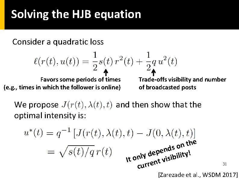
Solving the HJB equation Consider a quadratic loss Favors some periods of times (e. g. , times in which the follower is online) We propose optimal intensity is: Trade-offs visibility and number of broadcasted posts and then show that the n o s d n e ! ep y d t i y l l i n b isi It o v t n curre 31 [Zarezade et al. , WSDM 2017]

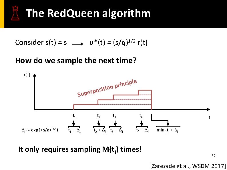
The Red. Queen algorithm Consider s(t) = s u*(t) = (s/q)1/2 r(t) How do we sample the next time? r(t) e pl i c n i r np io t i s o p Super t 1 Δi exp( (s/q)1/2 ) t 1 + Δ 1 t 2 t 3 t 2 + Δ 2 t 3 + Δ 3 t 4 + Δ 4 It only requires sampling M(tf) times! t mini ti + Δi 32 [Zarezade et al. , WSDM 2017]

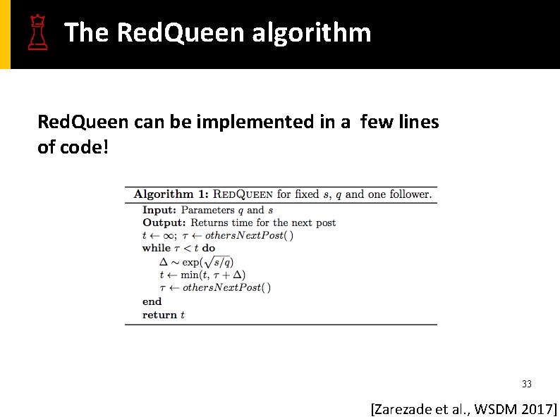
The Red. Queen algorithm Red. Queen can be implemented in a few lines of code! 33 [Zarezade et al. , WSDM 2017]

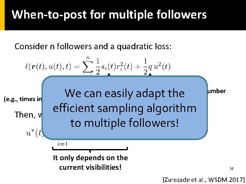
When-to-post for multiple followers Consider n followers and a quadratic loss: visibility and number We can easily Trade-offs adapt the of broadcasted posts efficient sampling algorithm Then, we can show that the optimal intensity is: to multiple followers! Favors some periods of times (e. g. , times in which the follower is online) It only depends on the current visibilities! 34 [Zarezade et al. , WSDM 2017]

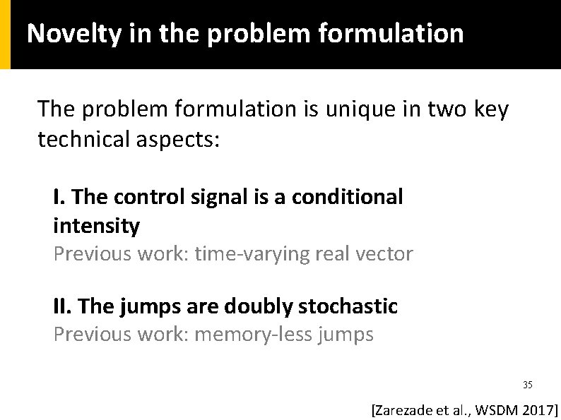
Novelty in the problem formulation The problem formulation is unique in two key technical aspects: I. The control signal is a conditional intensity Previous work: time-varying real vector II. The jumps are doubly stochastic Previous work: memory-less jumps 35 [Zarezade et al. , WSDM 2017]

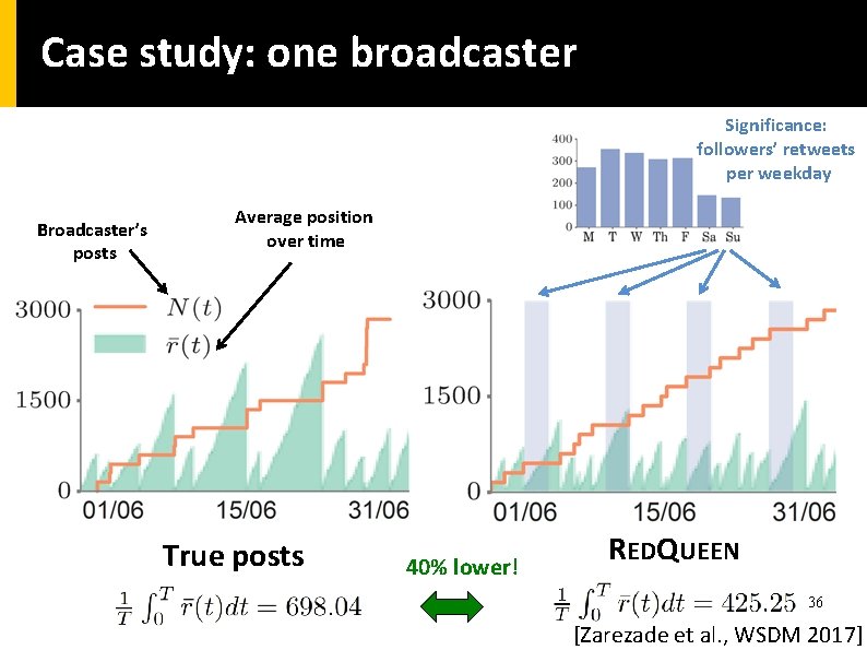
Case study: one broadcaster Significance: followers’ retweets per weekday Broadcaster’s posts Average position over time True posts 40% lower! REDQUEEN 36 [Zarezade et al. , WSDM 2017]

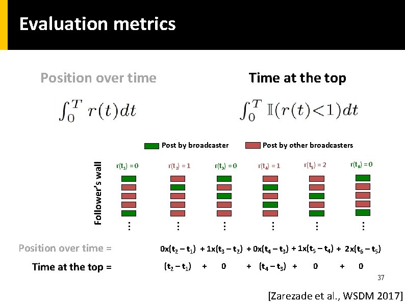
Evaluation metrics Position over time Time at the top r(t 3) = 0 Post by other broadcasters r(t 4) = 1 r(t 6) = 0 r(t 5) = 2 … … Time at the top = r(t 2) = 1 … Position over time = r(t 1) = 0 … Follower’s wall Post by broadcaster 0 x(t 2 – t 1) + 1 x(t 3 – t 2) + 0 x(t 4 – t 3) + 1 x(t 5 – t 4) + 2 x(t 6 – t 5) (t 2 – t 1) + 0 + (t 4 – t 3) + 0 37 [Zarezade et al. , WSDM 2017]

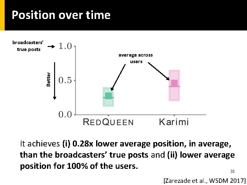
Position over time broadcasters’ true posts Better average across users It achieves (i) 0. 28 x lower average position, in average, than the broadcasters’ true posts and (ii) lower average position for 100% of the users. 38 [Zarezade et al. , WSDM 2017]

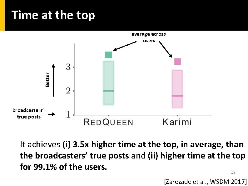
Time at the top Better average across users broadcasters’ true posts It achieves (i) 3. 5 x higher time at the top, in average, than the broadcasters’ true posts and (ii) higher time at the top for 99. 1% of the users. 39 [Zarezade et al. , WSDM 2017]

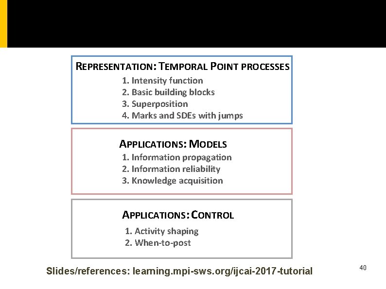
REPRESENTATION: TEMPORAL POINT PROCESSES 1. Intensity function 2. Basic building blocks 3. Superposition 4. Marks and SDEs with jumps APPLICATIONS: MODELS 1. Information propagation 2. Information reliability 3. Knowledge acquisition APPLICATIONS: CONTROL 1. Activity shaping 2. When-to-post Slides/references: learning. mpi-sws. org/ijcai-2017 -tutorial 40