Linear Systems Iterative Solutions CSE 541 Roger Crawfis

Linear Systems Iterative Solutions CSE 541 Roger Crawfis

Sparse Linear Systems Computational Science deals with the simulation of natural phenomenon, such as weather, blood flow, impact collision, earthquake response, etc. l To simulate these issues such as heat transfer, electromagnetic radiation, fluid flow and shock wave propagation need to be taken into account. l Combining initial conditions with general laws of physics (conservation of energy and mass), a model of these may involve a Partial Differential Equation (PDE). l

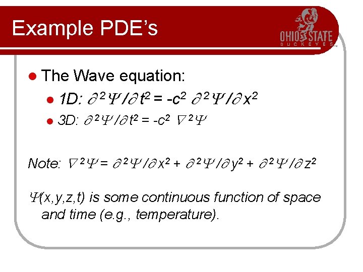
Example PDE’s l The Wave equation: l 1 D: 2 / t 2 = -c 2 2 / x 2 l 3 D: 2 / t 2 = -c 2 2 Note: 2 = 2 / x 2 + 2 / y 2 + 2 / z 2 (x, y, z, t) is some continuous function of space and time (e. g. , temperature).

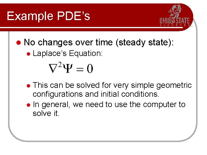
Example PDE’s l No l changes over time (steady state): Laplace’s Equation: This can be solved for very simple geometric configurations and initial conditions. l In general, we need to use the computer to solve it. l

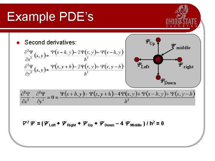
Example PDE’s l Second derivatives: Up middle Left right Down 2 = ( Left + Right + Up + Down – 4 Middle ) / h 2 = 0

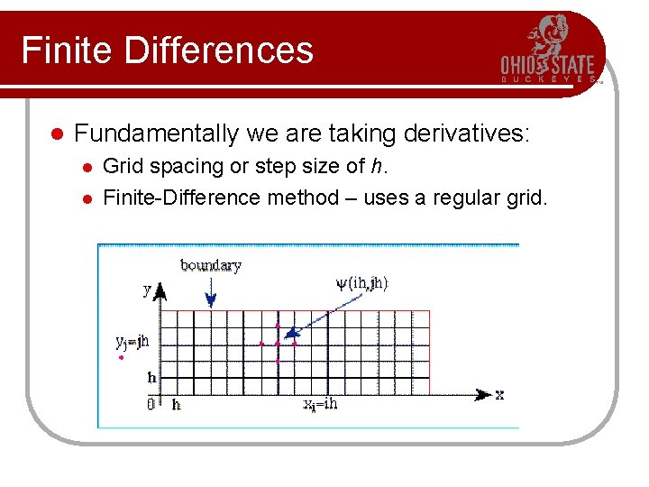
Finite Differences l Fundamentally we are taking derivatives: l l Grid spacing or step size of h. Finite-Difference method – uses a regular grid.

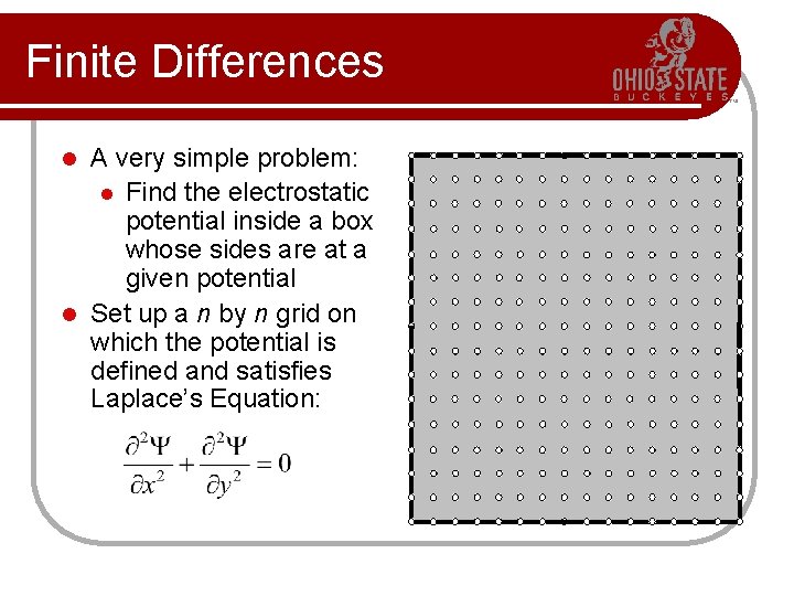
Finite Differences A very simple problem: l Find the electrostatic potential inside a box whose sides are at a given potential l Set up a n by n grid on which the potential is defined and satisfies Laplace’s Equation: l

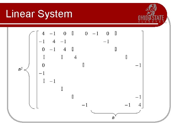
Linear System n 2 n

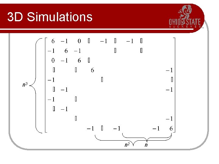
3 D Simulations n 3 n 2 n

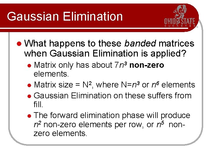
Gaussian Elimination l What happens to these banded matrices when Gaussian Elimination is applied? Matrix only has about 7 n 3 non-zero elements. l Matrix size = N 2, where N=n 3 or n 6 elements l Gaussian Elimination on these suffers from fill. l The forward elimination phase will produce n 2 non-zero elements per row, or n 5 nonzero elements. l

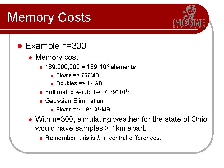
Memory Costs l Example n=300 l Memory cost: l 189, 000 = 189*106 elements l l Full matrix would be: 7. 29*1014! Gaussian Elimination l l Floats => 756 MB Doubles => 1. 4 GB Floats => 1. 9*1013 MB With n=300, simulating weather for the state of Ohio would have samples > 1 km apart. l Remember, this is h in central differences.

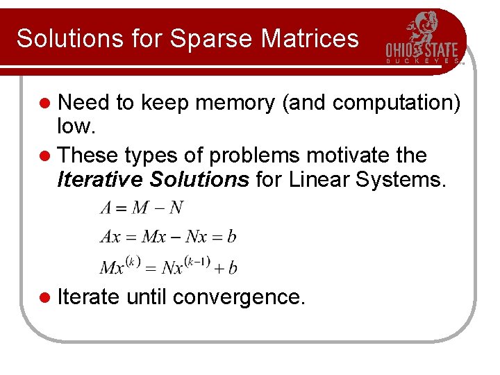
Solutions for Sparse Matrices l Need to keep memory (and computation) low. l These types of problems motivate the Iterative Solutions for Linear Systems. l Iterate until convergence.

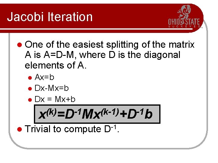
Jacobi Iteration l One of the easiest splitting of the matrix A is A=D-M, where D is the diagonal elements of A. Ax=b l Dx-Mx=b l Dx = Mx+b x(k)=D-1 Mx(k-1)+D-1 b l l Trivial to compute D-1.

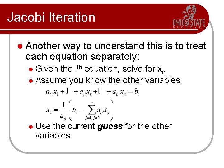
Jacobi Iteration l Another way to understand this is to treat each equation separately: Given the ith equation, solve for xi. l Assume you know the other variables. l l Use the current guess for the other variables.

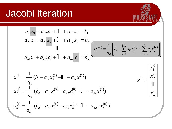
Jacobi iteration

Jacobi Iteration l Cute, but will it work? l Algorithms, even mathematical ones, need a mathematical framework or analysis. l Let’s first look at a simple example.

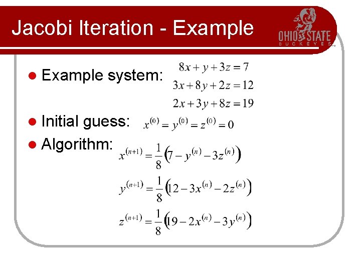
Jacobi Iteration - Example l Initial system: guess: l Algorithm:

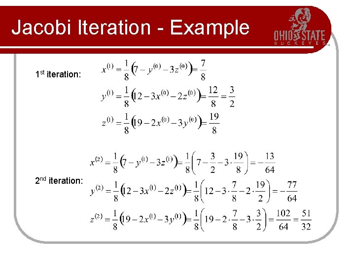
Jacobi Iteration - Example 1 st iteration: 2 nd iteration:

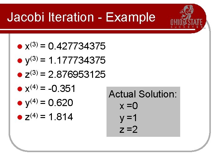
Jacobi Iteration - Example l x(3) = 0. 427734375 l y(3) = 1. 177734375 l z(3) = 2. 876953125 l x(4) = -0. 351 Actual Solution: l y(4) = 0. 620 x =0 l z(4) = 1. 814 y =1 z =2

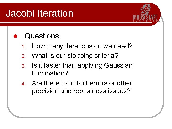
Jacobi Iteration l Questions: 1. 2. 3. 4. How many iterations do we need? What is our stopping criteria? Is it faster than applying Gaussian Elimination? Are there round-off errors or other precision and robustness issues?

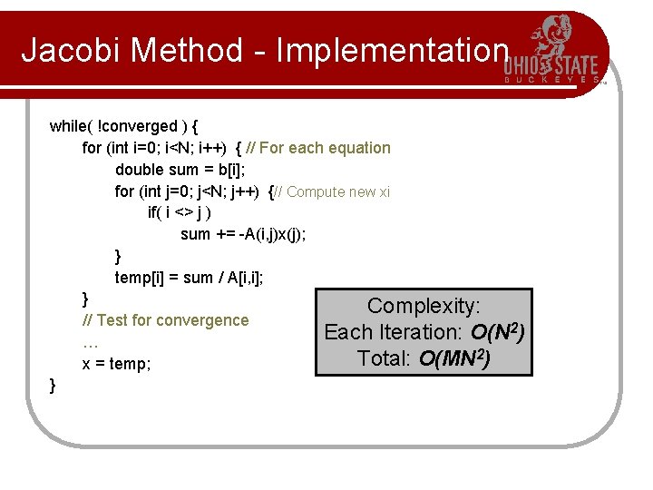
Jacobi Method - Implementation while( !converged ) { for (int i=0; i<N; i++) { // For each equation double sum = b[i]; for (int j=0; j<N; j++) {// Compute new xi if( i <> j ) sum += -A(i, j)x(j); } temp[i] = sum / A[i, i]; } Complexity: // Test for convergence 2) Each Iteration: O(N … Total: O(MN 2) x = temp; }

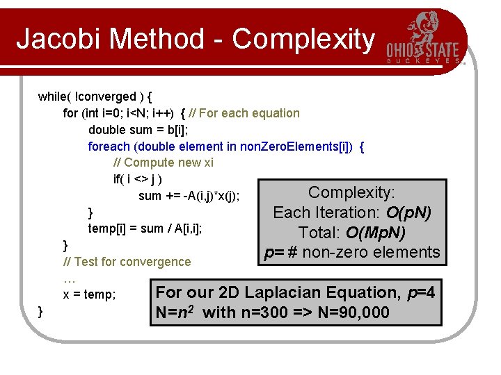
Jacobi Method - Complexity while( !converged ) { for (int i=0; i<N; i++) { // For each equation double sum = b[i]; foreach (double element in non. Zero. Elements[i]) { // Compute new xi if( i <> j ) Complexity: sum += -A(i, j)*x(j); } Each Iteration: O(p. N) temp[i] = sum / A[i, i]; Total: O(Mp. N) } p= # non-zero elements // Test for convergence … For our 2 D Laplacian Equation, p=4 x = temp; } N=n 2 with n=300 => N=90, 000

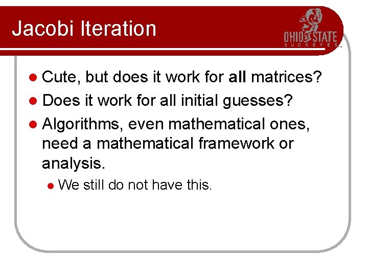
Jacobi Iteration l Cute, but does it work for all matrices? l Does it work for all initial guesses? l Algorithms, even mathematical ones, need a mathematical framework or analysis. l We still do not have this.

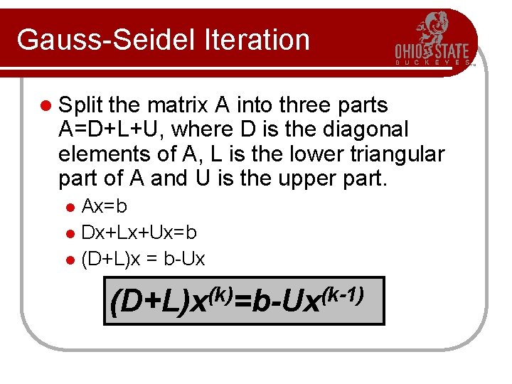
Gauss-Seidel Iteration l Split the matrix A into three parts A=D+L+U, where D is the diagonal elements of A, L is the lower triangular part of A and U is the upper part. Ax=b l Dx+Lx+Ux=b l (D+L)x = b-Ux l (D+L)x(k)=b-Ux(k-1)

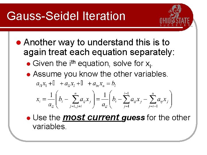
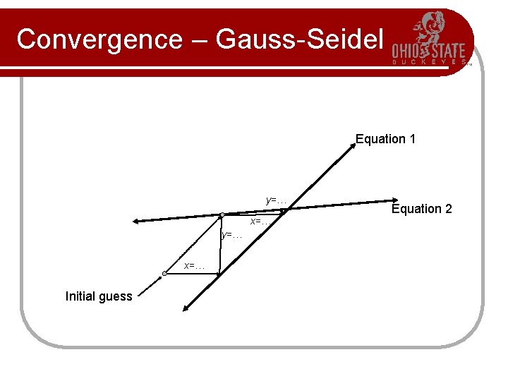
Gauss-Seidel Iteration l Another way to understand this is to again treat each equation separately: Given the ith equation, solve for xi. l Assume you know the other variables. l l Use the most current guess for the other variables.

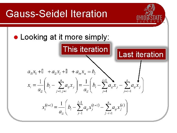
Gauss-Seidel Iteration l Looking at it more simply: This iteration Last iteration

Gauss-Seidel Iteration l Questions: 1. 2. 3. 4. How many iterations do we need? What is our stopping criteria? Is it faster than applying Gaussian Elimination? Are there round-off errors or other precision and robustness issues?

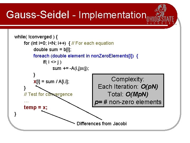
Gauss-Seidel - Implementation while( !converged ) { for (int i=0; i<N; i++) { // For each equation double sum = b[i]; foreach (double element in non. Zero. Elements[i]) { if( i <> j ) sum += -A(i, j)x(j); } Complexity: x[i] = sum / A[i, i]; Each Iteration: O(p. N) } // Test for convergence Total: O(Mp. N) … p= # non-zero elements temp = x; } Differences from Jacobi

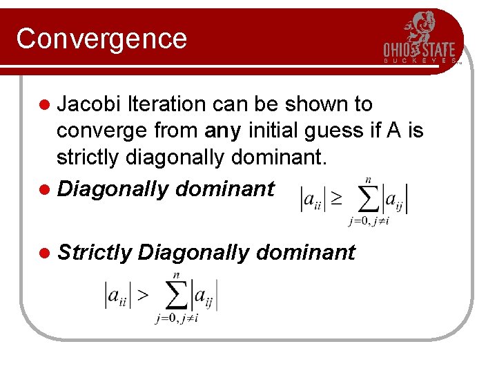
Convergence l Jacobi Iteration can be shown to converge from any initial guess if A is strictly diagonally dominant. l Diagonally dominant l Strictly Diagonally dominant

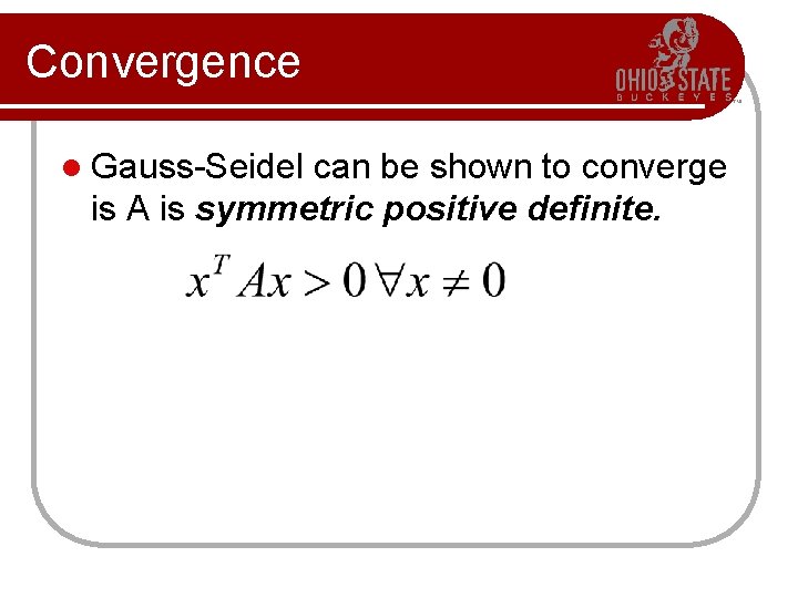
Convergence l Gauss-Seidel can be shown to converge is A is symmetric positive definite.

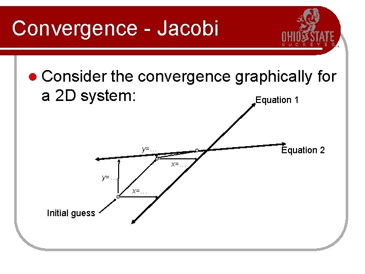
Convergence - Jacobi l Consider the convergence graphically for a 2 D system: Equation 1 Equation 2 y=… x=… Initial guess

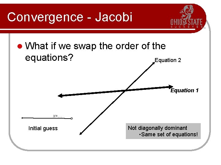
Convergence - Jacobi l What if we swap the order of the equations? Equation 2 Equation 1 x=… Initial guess Not diagonally dominant • Same set of equations!

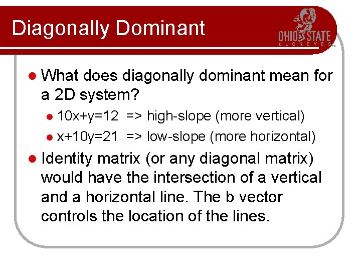
Diagonally Dominant l What does diagonally dominant mean for a 2 D system? 10 x+y=12 => high-slope (more vertical) l x+10 y=21 => low-slope (more horizontal) l l Identity matrix (or any diagonal matrix) would have the intersection of a vertical and a horizontal line. The b vector controls the location of the lines.

Convergence – Gauss-Seidel Equation 1 y=… x=… Initial guess Equation 2

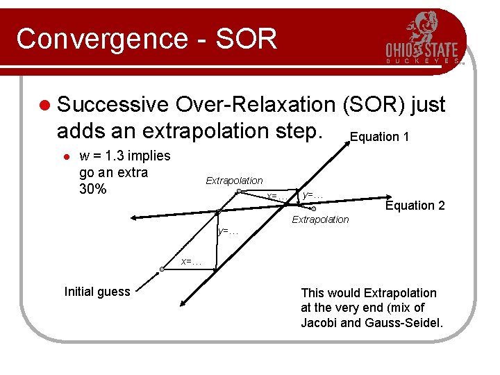
Convergence - SOR l Successive Over-Relaxation (SOR) just adds an extrapolation step. Equation 1 l w = 1. 3 implies go an extra 30% Extrapolation x=… y=… Equation 2 Extrapolation y=… x=… Initial guess This would Extrapolation at the very end (mix of Jacobi and Gauss-Seidel.

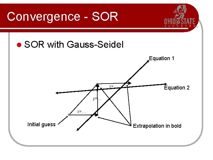
Convergence - SOR l SOR with Gauss-Seidel Equation 1 x=… Equation 2 y=… x=… Initial guess Extrapolation in bold