Linear Systems LU Factorization CSE 541 Roger Crawfis
- Slides: 19

Linear Systems LU Factorization CSE 541 Roger Crawfis

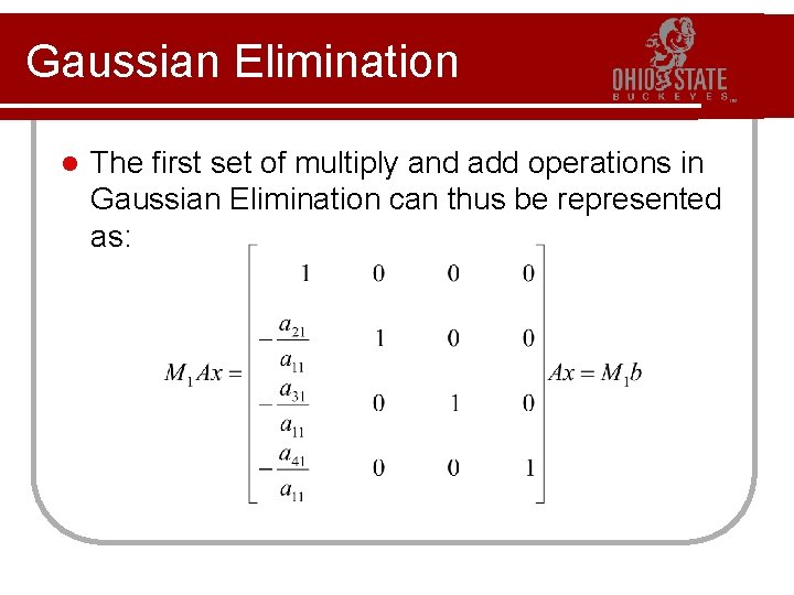
Gaussian Elimination l We are going to look at the algorithm for Gaussian Elimination as a sequence of matrix operations (multiplies). l Not really how you want to implement it, but gives a better framework for theory, and our next topic: l LU-factorization.

Permutations l. A permutation matrix P is a re-ordering of the identity matrix I. It can be used to: l Interchange the order of the equations l l Interchange the rows of A and b Interchange the order of the variables This technique changes the order of the solution variables. l Hence a reordering is required after the solution is found. l

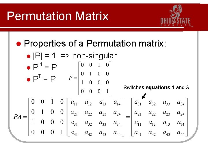
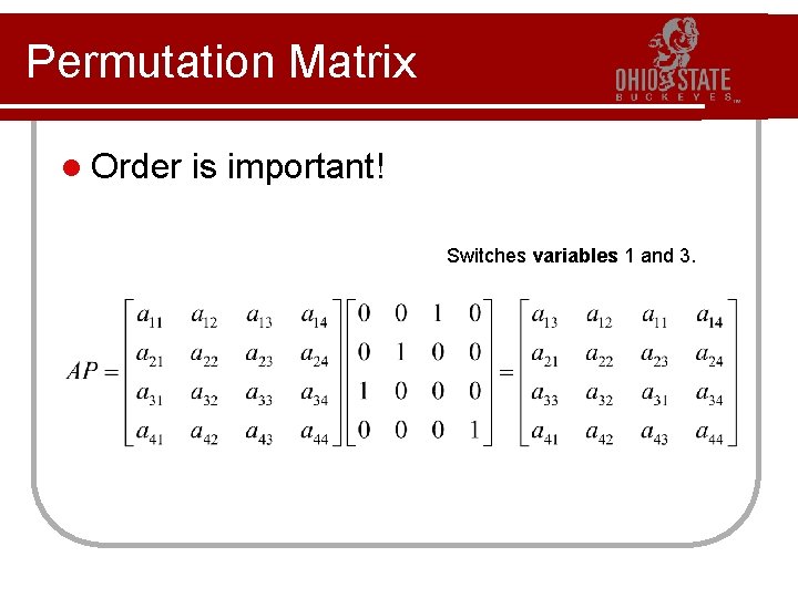
Permutation Matrix l Properties of a Permutation matrix: |P| = 1 => non-singular -1 l. P =P T l. P =P l Switches equations 1 and 3.

Permutation Matrix l Order is important! Switches variables 1 and 3.

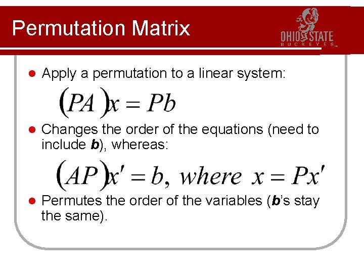
Permutation Matrix l Apply a permutation to a linear system: l Changes the order of the equations (need to include b), whereas: l Permutes the order of the variables (b’s stay the same).

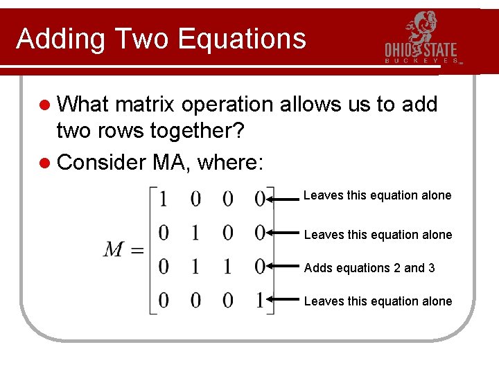
Adding Two Equations l What matrix operation allows us to add two rows together? l Consider MA, where: Leaves this equation alone Adds equations 2 and 3 Leaves this equation alone

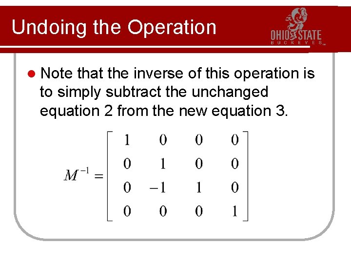
Undoing the Operation l Note that the inverse of this operation is to simply subtract the unchanged equation 2 from the new equation 3.

Gaussian Elimination l The first set of multiply and add operations in Gaussian Elimination can thus be represented as:

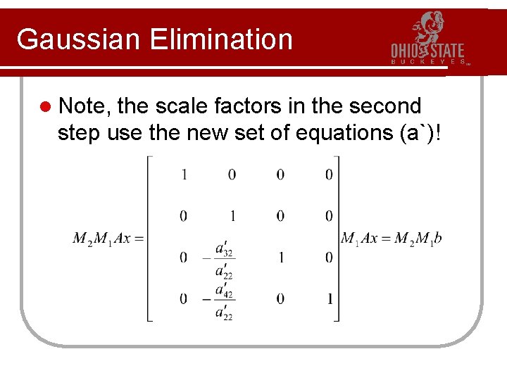
Gaussian Elimination l Note, the scale factors in the second step use the new set of equations (a`)!

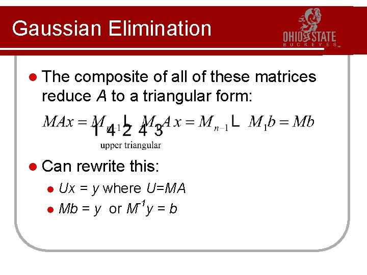
Gaussian Elimination l The composite of all of these matrices reduce A to a triangular form: l Can rewrite this: Ux = y where U=MA -1 l Mb = y or M y = b l

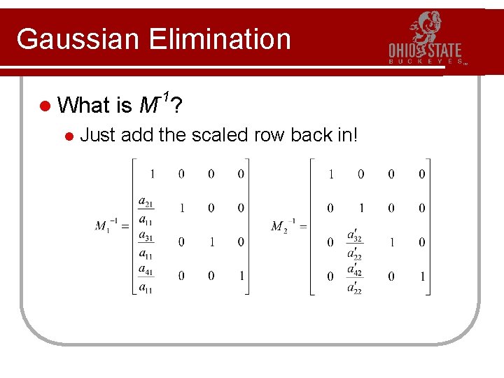
Gaussian Elimination l What l -1 is M ? Just add the scaled row back in!

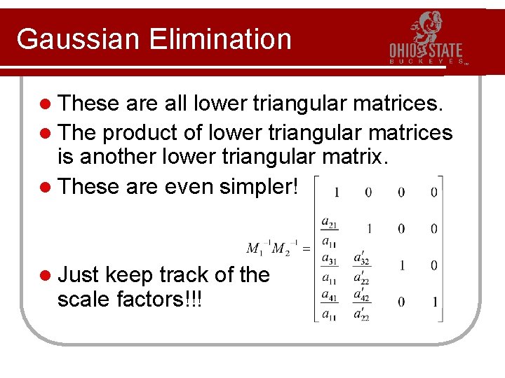
Gaussian Elimination l These are all lower triangular matrices. l The product of lower triangular matrices is another lower triangular matrix. l These are even simpler! l Just keep track of the scale factors!!!

LU Factorization l Let -1 L = M and U = MA L is a lower triangular matrix with 1’s on the diagonal. l U is an upper triangular matrix: l l Given these, we can trivially solve (in O(n 2) time): Ly = b – forward substitution l Ux = y – backward substitution l

LU Factorization l Note, l L and U are only dependent on A. A = LU – a factorization of A l Hence, Ax=b implies LUx = b or l Ly = b where Ux = y l Find y and then we can solve for x. l Both operations in O(n 2) time. l

LU Factorization l Problem: How do we compute the LU factorization? l Answer: Gaussian Elimination l Which is O(n 3) time, so no free lunch!

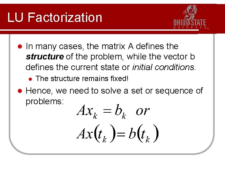
LU Factorization l In many cases, the matrix A defines the structure of the problem, while the vector b defines the current state or initial conditions. l l The structure remains fixed! Hence, we need to solve a set or sequence of problems:

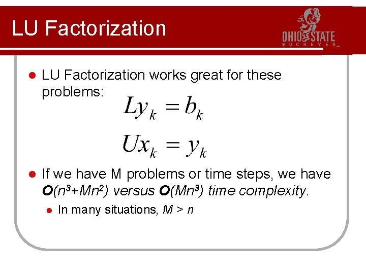
LU Factorization l LU Factorization works great for these problems: l If we have M problems or time steps, we have O(n 3+Mn 2) versus O(Mn 3) time complexity. l In many situations, M > n

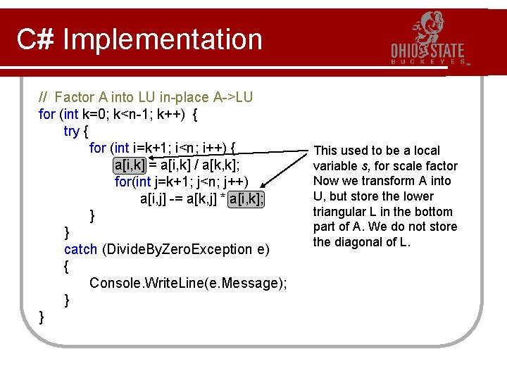
C# Implementation // Factor A into LU in-place A->LU for (int k=0; k<n-1; k++) { try { for (int i=k+1; i<n; i++) { a[i, k] = a[i, k] / a[k, k]; for(int j=k+1; j<n; j++) a[i, j] -= a[k, j] * a[i, k]; } } catch (Divide. By. Zero. Exception e) { Console. Write. Line(e. Message); } } This used to be a local variable s, for scale factor Now we transform A into U, but store the lower triangular L in the bottom part of A. We do not store the diagonal of L.