Chapter 3 States and Searching Uninformed Search Techniques

Chapter 3: States and Searching: Uninformed Search Techniques Textbook: Artificial Intelligence Foundations of Computational Agents, 2 nd Edition, David L. Poole and Alan K Mackworth, Cambridge University Press, 2018. Asst. Prof. Dr. Anilkumar K. G 1

Learning Objectives • At the end of the class you should be able to: – define a directed graph – represent a problem as a state-space graph – explain how a generic searching algorithm works on a uninformed search problem Asst. Prof. Dr. Anilkumar K. G 2

Topic Overview • The previous chapter discussed about how an agent perceives and acts in its environment. • An agent could be programmed to act in the world to achieve a fixed set of goals, but if it may not adapt to changing goals then it would not be intelligent. • This chapter shows how the problem of an agent deciding what to do can be cast as the problem of searching to find a path in a graph. • Searching means searching in an internal representation for a path to a given goal. Asst. Prof. Dr. Anilkumar K. G 3

Problem Solving as Search • An agent could be programmed to act in the world to achieve its goal states – An intelligent agent needs to reason about its abilities and its goals to determine what to do – This section describes how an agent can find its goal path by searching a problem space depicted as a graph. • In the simplest, an agent deciding what it should do, – the agent has a state-based model of the world with a goal state to achieve its goal path without uncertainty • The agent is able to determine how to achieve its goal path by searching in its representation of the world state space for a way to get from its current state to a goal state. Asst. Prof. Dr. Anilkumar K. G 4

Problem Solving as Search • The searching problem can be abstracted to a mathematical problem of finding a path from the start node to a goal node in a directed graph – Search proceeds by repeatedly selecting a partial solution, stopping if it is a path to a goal, – and otherwise extending it by one more arc in all possible ways. • To solve some search problems efficiently, – agents should exploit special knowledge about domain to guide them to a solution. – This extra knowledge beyond the search space is heuristic knowledge. Asst. Prof. Dr. Anilkumar K. G 5

State Spaces • One general formulation of intelligent action is in terms of a state space (problem space) • A state contains all of the information necessary to predict the effects of an action and to determine a goal state – the agent has perfect knowledge of the state space and can observe what state it is in (full observability) – the agent has a set of actions that have known deterministic effects – The agent can determine whether a state satisfies the goal • A solution is a sequence of actions from current state to a state that satisfies the goal. Asst. Prof. Dr. Anilkumar K. G 6

State Spaces • A state-space consists of – a set of states – a distinguished state called the start state – for each state, a set of actions available to the agent in that state an action function that returns a new state value – a goal state, s is specified by a Boolean function, goal(s) when the state s satisfies the goal criteria • A criterion that specifies the quality of the acceptable solution – For example, the goal state of an agent may be acceptable, only when its goal related sequence end up with a minimal total cost. Asst. Prof. Dr. Anilkumar K. G 7

Graph Searching • The problem of finding a sequence of actions to achieve a goal is abstracted as searching for paths in directed graphs – To solve a problem, first define the underlying search space and then apply a search algorithm to the search space – A directed graph consists of a set of nodes and a set of directed arcs between nodes – The search idea is to find a path along these arcs from a start node to a goal node • In representing a state-space problem, the states are represented as nodes, and the actions as arcs Asst. Prof. Dr. Anilkumar K. G 8

Formalizing Graph Searching • A directed graph consists of: – a set of N nodes and – a set of A arcs, where an arc is an ordered pairs of nodes – The arc (n 1, n 2) is an outgoing arc from n 1 and an incoming arc to n 2 ; where (n 1, n 2 ) ∈ A (where A is a set of arcs). – A node n 2 is a neighbor of n 1 if there is an arc from n 1 to n 2 – A path from node s to node g is a sequence of nodes {n 0, n 1, . . . , nk} such that s = n 0, g = nk – A Boolean function on goal(n) is true, then n is a goal node Asst. Prof. Dr. Anilkumar K. G 9

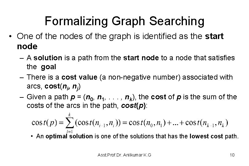
Formalizing Graph Searching • One of the nodes of the graph is identified as the start node – A solution is a path from the start node to a node that satisfies the goal – There is a cost value (a non-negative number) associated with arcs, cost(ni, nj) – Given a path p = (n 0, n 1, . . . , nk), the cost of p is the sum of the costs of the arcs in the path, cost(p): • An optimal solution is one of the solutions that has the lowest cost path. Asst. Prof. Dr. Anilkumar K. G 10

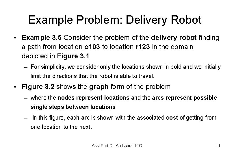
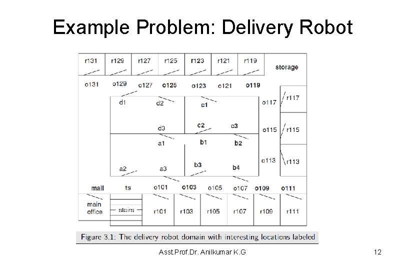
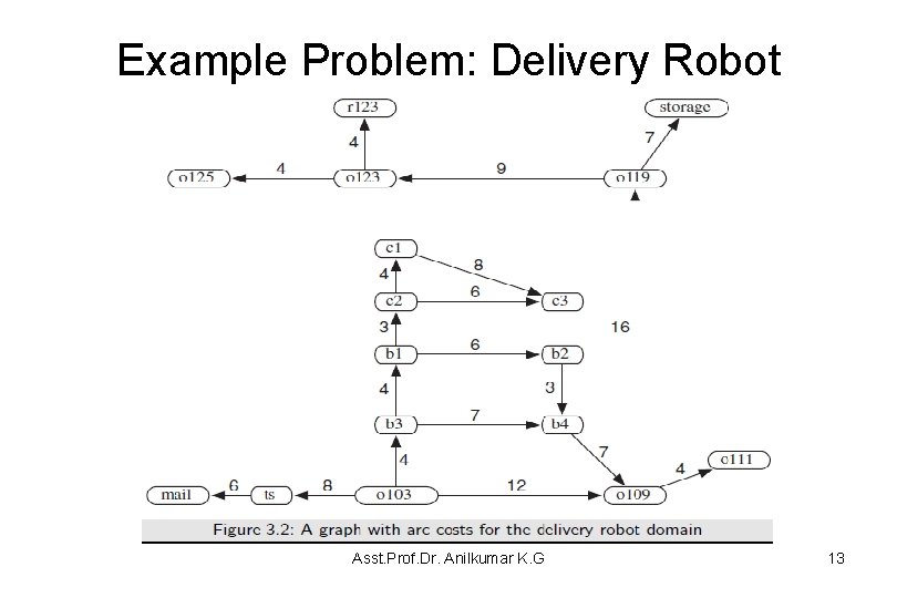
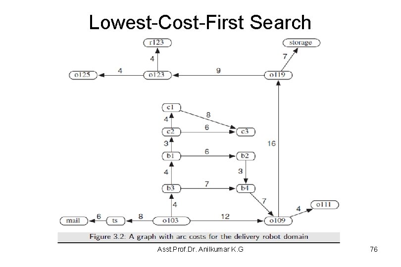
Example Problem: Delivery Robot • Example 3. 5 Consider the problem of the delivery robot finding a path from location o 103 to location r 123 in the domain depicted in Figure 3. 1 – For simplicity, we consider only the locations shown in bold and we initially limit the directions that the robot is able to travel. • Figure 3. 2 shows the graph form of the problem – where the nodes represent locations and the arcs represent possible single steps between locations – In this figure, each arc is shown with the associated cost of getting from one location to the next. Asst. Prof. Dr. Anilkumar K. G 11

Example Problem: Delivery Robot Asst. Prof. Dr. Anilkumar K. G 12

Example Problem: Delivery Robot Asst. Prof. Dr. Anilkumar K. G 13

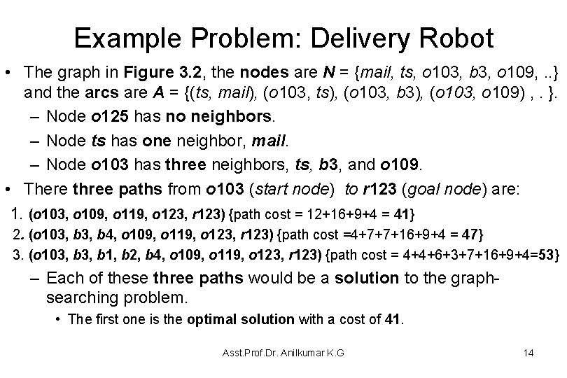
Example Problem: Delivery Robot • The graph in Figure 3. 2, the nodes are N = {mail, ts, o 103, b 3, o 109, . . } and the arcs are A = {(ts, mail), (o 103, ts), (o 103, b 3), (o 103, o 109) , . }. – Node o 125 has no neighbors. – Node ts has one neighbor, mail. – Node o 103 has three neighbors, ts, b 3, and o 109. • There three paths from o 103 (start node) to r 123 (goal node) are: 1. (o 103, o 109, o 119, o 123, r 123) {path cost = 12+16+9+4 = 41} 2. (o 103, b 4, o 109, o 119, o 123, r 123) {path cost =4+7+7+16+9+4 = 47} 3. (o 103, b 1, b 2, b 4, o 109, o 119, o 123, r 123) {path cost = 4+4+6+3+7+16+9+4=53} – Each of these three paths would be a solution to the graphsearching problem. • The first one is the optimal solution with a cost of 41. Asst. Prof. Dr. Anilkumar K. G 14

Graph Searching • A cycle is a nonempty path such that the end node is the same as the start node – A cycle is a path (n 0, n 1, . . . , nk) such that n 0 = nk • A directed graph without any cycles is called a directed acyclic graph (DAG) – A tree is a DAG where there is one node with no incoming arcs and every other node has exactly one incoming arc. – The start node is called the root of the tree and nodes with no outgoing arcs are called leaves. – In a tree, neighbors are called children • In many problems the search graph is not given explicitly. For a search algorithms it is require to generate search space to determine if the node is a goal node. Asst. Prof. Dr. Anilkumar K. G 15

Graph Searching • The forward branching factor of a node is the number of arcs leaving the node – in the graph in Figure 3. 2, the forward branching factor of node o 103 is 3 (there are 3 arcs coming out of the node o 103) and mail is 0. • The backward branching factor of a node is the number of arcs entering the node – The backward branching factor of node o 103 is 0 (there are no arcs coming into node o 103). The backward branching factor of mail is 1. • These branching factors provide measures for the complexity of graph algorithms – Bounded branching factors are assumed when estimating the time and space complexities of search algorithms Asst. Prof. Dr. Anilkumar K. G 16

Graph Searching • The branching factor is important because it is a key component in the size of the graph. • If the forward branching factor of each node is b, and the graph is a tree, then there are bn nodes that are n arcs away from any node. Asst. Prof. Dr. Anilkumar K. G 17

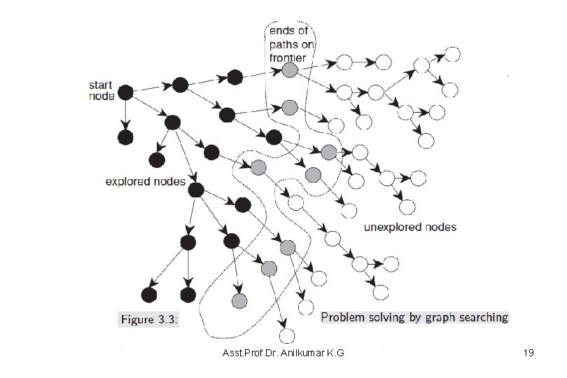
A Generic Searching Algorithm • A generic graph search algorithm to search for a solution path in a graph is described – The idea behind the generic graph search algorithm is, the given graph has a start node, and a goal node, • It is to explore paths incrementally from the start node – This is done by maintaining a frontier (or a list) of paths from the start node (see Figure 3. 3) – The frontier contains all of the paths from the start node to a goal node • Initially, the frontier contains just the start node • As the search proceeds, the frontier expands into unexplored nodes until a goal node is encountered Asst. Prof. Dr. Anilkumar K. G 18

Asst. Prof. Dr. Anilkumar K. G 19

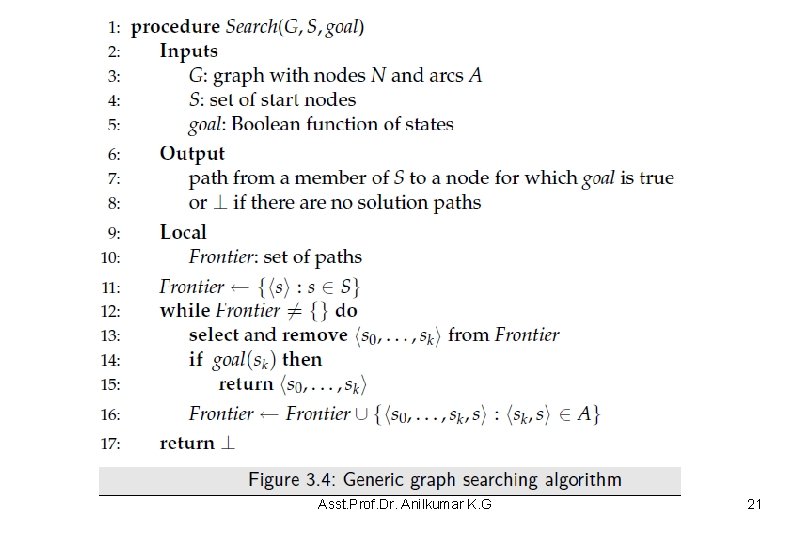
A Generic Searching Algorithm • The generic search algorithm is shown in Figure 3. 4. • Initially, the frontier just a start node with zero path cost: – At each step, the algorithm removes a path (n 0, . . . , nk) from the frontier – If goal(nk) is true (nk is a goal node), it has found a solution and returns the solution path (n 0, . . , nk) – Otherwise, the path is extended by one more arc by finding the neighbors of nk – For every neighbor n of nk, the path (n 0, . . . , nk, n) is added to the frontier • This step is known as expanding the path node (n 0, . . . , nk) Asst. Prof. Dr. Anilkumar K. G 20

Asst. Prof. Dr. Anilkumar K. G 21

A Generic Searching Algorithm • If the node at the end of the selected path is not a goal node, and it has no neighbors, then extending the path means removing the path from the frontier • A graph problem determines the goal but not select a goal path from the frontier – This is the job of a search strategy • A search strategy defines the order in which paths are selected from the frontier. Asst. Prof. Dr. Anilkumar K. G 22

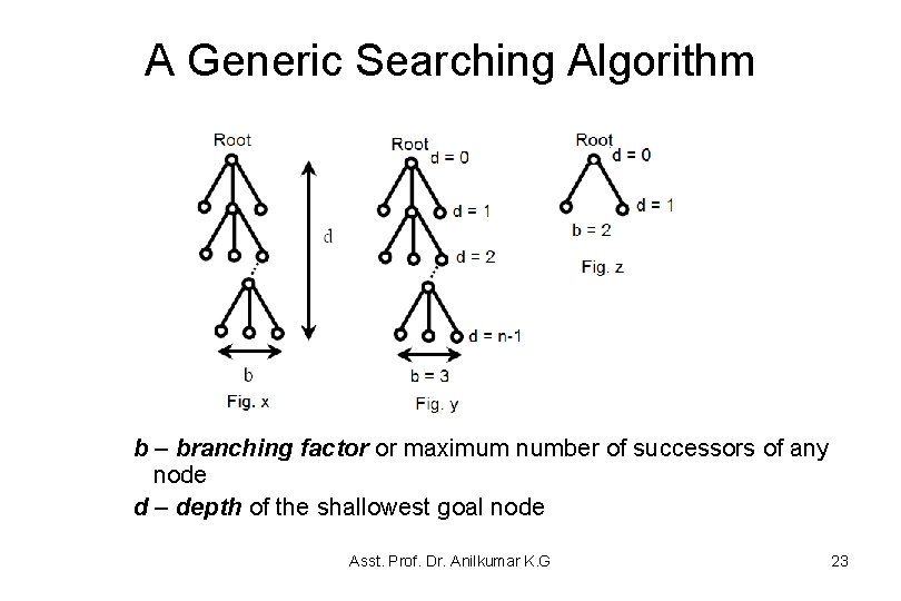
A Generic Searching Algorithm b – branching factor or maximum number of successors of any node d – depth of the shallowest goal node Asst. Prof. Dr. Anilkumar K. G 23

A Generic Searching Algorithm • Evaluate the performance of a search algorithm in four ways: Completeness: Does it guarantee to find a solution if one exists? Time complexity: How long does it find a solution? (It indicates the number of node generation by the algorithm) Space complexity: How much memory needed to perform the search? Optimality: Does the strategy find an optimal solution? • Time and space complexity are measured in terms of: b – branching factor or maximum number of successors of any node d or k– depth of the shallowest goal node m – maximum length of any path in the state space (may be infinite) Asst. Prof. Dr. Anilkumar K. G 24

Uninformed Search Strategies • This section presents four uninformed search strategies that do not take into account the location of the goal 1. 2. 3. 4. • Breadth-first Search Depth-first Search Iterative Deepening Search Lowest-cost-first Search Intuitively, these algorithms ignore where they are going until they find a goal and report success Asst. Prof. Dr. Anilkumar K. G 25

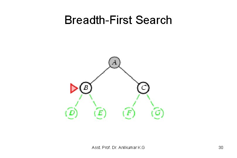
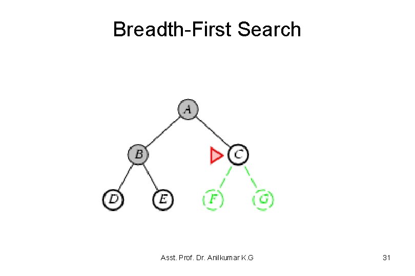
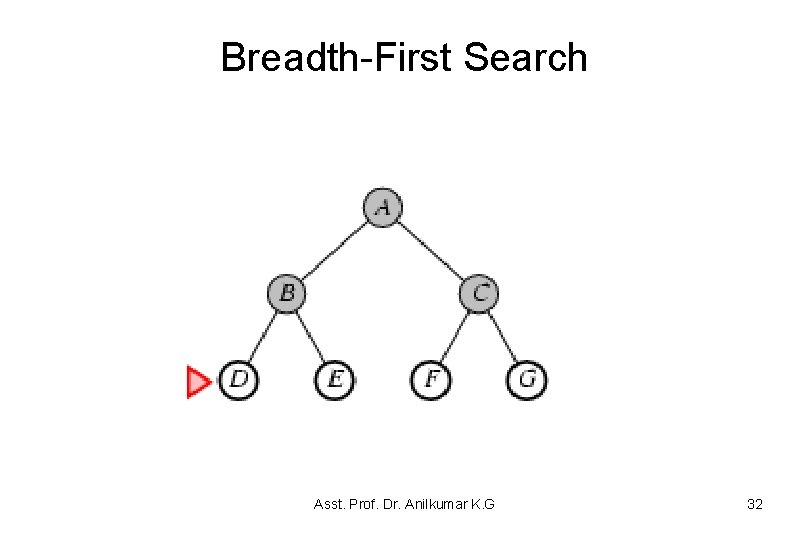
Breadth-First Search • In breadth-first search the frontier is implemented as a FIFO (first-in, first-out) queue – Thus, the path that is selected from the frontier is the one that was added earliest • This approach implies that the paths from the start node are generated in order of the number of arcs in the path. • One of the paths with the fewest arcs is selected at each iteration stage. Asst. Prof. Dr. Anilkumar K. G 26

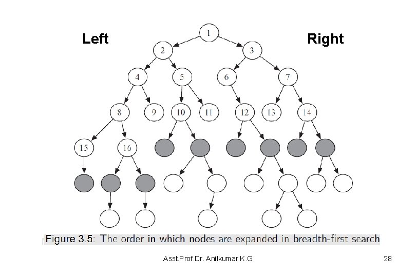
Breadth-First Search • Consider the graph in Figure 3. 5 – Suppose the start node is the node at the top (node 1), and the children of a node are added to left-to-right order. – In breadth-first search, as in depth-first search, the order in which the nodes are expanded does not depend on the location of the goal – The nodes at the end of the first sixteen paths expanded are numbered in the order of their expansion (see Figure 3. 5). – The shaded nodes are the nodes at the ends of the paths of the frontier after the first sixteen steps/iteration. Asst. Prof. Dr. Anilkumar K. G 27

Left Right Asst. Prof. Dr. Anilkumar K. G 28

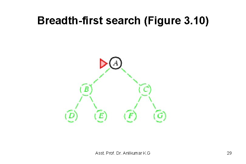
Breadth-first search (Figure 3. 10) Asst. Prof. Dr. Anilkumar K. G 29

Breadth-First Search Asst. Prof. Dr. Anilkumar K. G 30

Breadth-First Search Asst. Prof. Dr. Anilkumar K. G 31

Breadth-First Search Asst. Prof. Dr. Anilkumar K. G 32

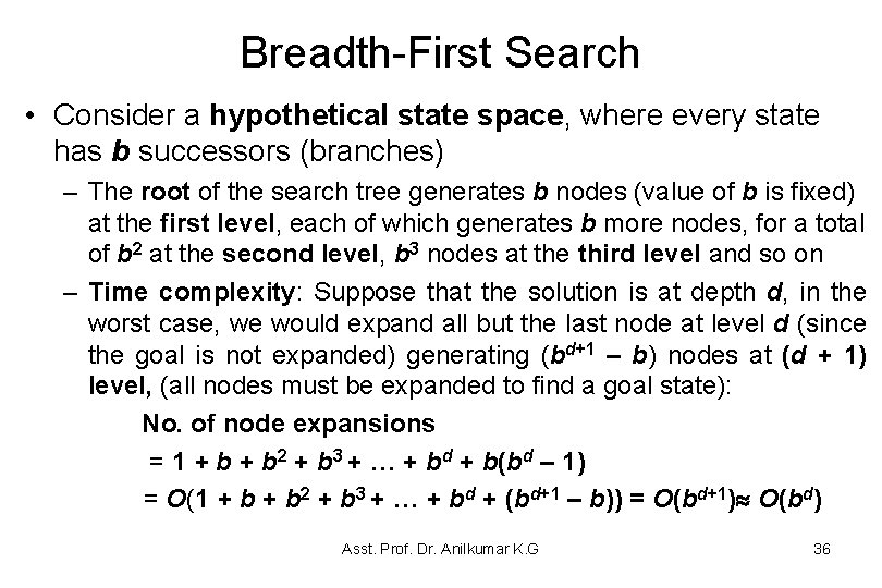
Breadth-First Search • The search procedure: List CLOSED = [Empty], OPEN = [Start Node] Loop: If OPEN = NULL, stop // No goal. Else, set N = OPEN[0] If N is goal , then stop //Solution else, remove N from OPEN If N is in CLOSED, then Goto Loop Else, append N to CLOSED Append any children of N to OPEN Goto Loop. • Convention is that nodes are ordered ‘left to right’ Asst. Prof. Dr. Anilkumar K. G 33

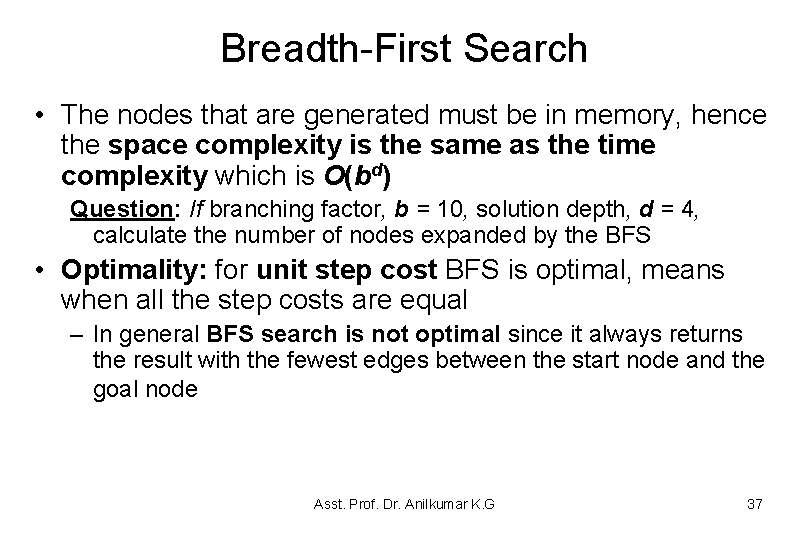
Breadth-First Search {frontier[] = OPEN[]} Asst. Prof. Dr. Anilkumar K. G 34

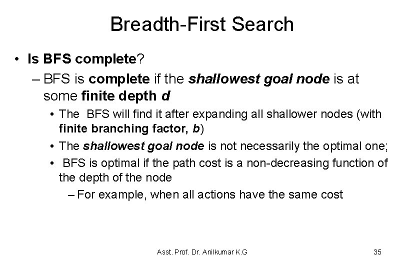
Breadth-First Search • Is BFS complete? – BFS is complete if the shallowest goal node is at some finite depth d • The BFS will find it after expanding all shallower nodes (with finite branching factor, b) • The shallowest goal node is not necessarily the optimal one; • BFS is optimal if the path cost is a non-decreasing function of the depth of the node – For example, when all actions have the same cost Asst. Prof. Dr. Anilkumar K. G 35

Breadth-First Search • Consider a hypothetical state space, where every state has b successors (branches) – The root of the search tree generates b nodes (value of b is fixed) at the first level, each of which generates b more nodes, for a total of b 2 at the second level, b 3 nodes at the third level and so on – Time complexity: Suppose that the solution is at depth d, in the worst case, we would expand all but the last node at level d (since the goal is not expanded) generating (bd+1 – b) nodes at (d + 1) level, (all nodes must be expanded to find a goal state): No. of node expansions = 1 + b 2 + b 3 + … + bd + b(bd – 1) = O(1 + b 2 + b 3 + … + bd + (bd+1 – b)) = O(bd+1) O(bd) Asst. Prof. Dr. Anilkumar K. G 36

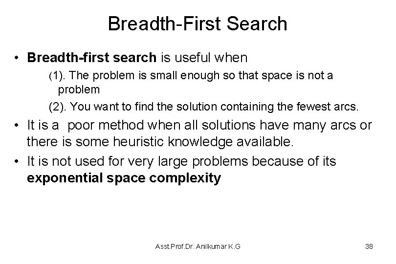
Breadth-First Search • The nodes that are generated must be in memory, hence the space complexity is the same as the time complexity which is O(bd) Question: If branching factor, b = 10, solution depth, d = 4, calculate the number of nodes expanded by the BFS • Optimality: for unit step cost BFS is optimal, means when all the step costs are equal – In general BFS search is not optimal since it always returns the result with the fewest edges between the start node and the goal node Asst. Prof. Dr. Anilkumar K. G 37

Breadth-First Search • Breadth-first search is useful when (1). The problem is small enough so that space is not a problem (2). You want to find the solution containing the fewest arcs. • It is a poor method when all solutions have many arcs or there is some heuristic knowledge available. • It is not used for very large problems because of its exponential space complexity Asst. Prof. Dr. Anilkumar K. G 38

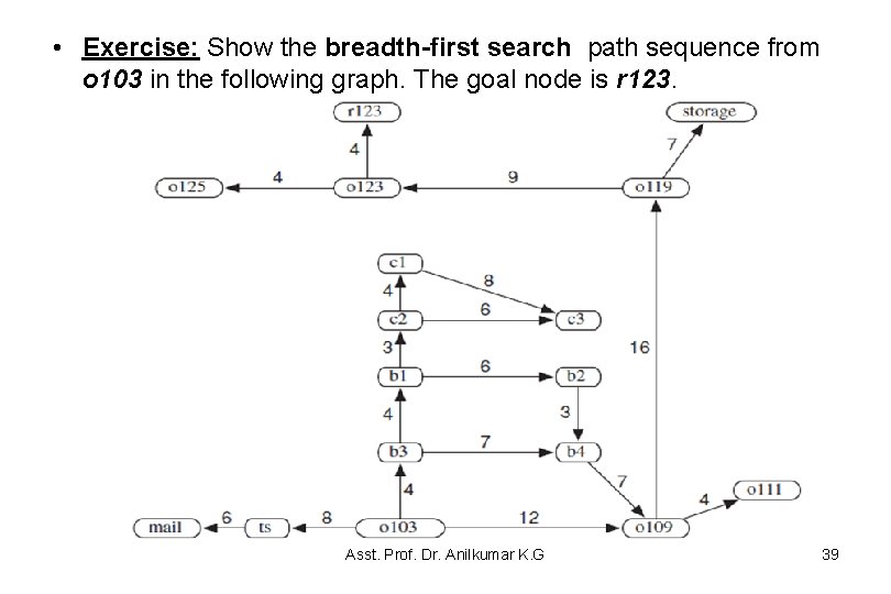
• Exercise: Show the breadth-first search path sequence from o 103 in the following graph. The goal node is r 123. Asst. Prof. Dr. Anilkumar K. G 39

1. Open[o 103] Closed[] 2. Open[ts, b 3, o 109] Closed[o 103] 3. Open[b 3, o 109, mail] Closed[o 103, ts] 4. Open[o 109, mail, b 1, b 4] Closed[o 103, ts, b 3] 5. Open[mail, b 1, b 4, o 119, o 111] Closed[o 103, ts, b 3, o 109] 6. Open[b 1, b 4, o 119, o 111] Closed[o 103, ts, b 3, o 109, mail] 7. Open[b 4, o 119, o 111, c 2, b 2] Closed[o 103, ts, b 3, o 109, mail, b 1] 8. Open[o 119, o 111, c 2, b 2] Closed[o 103, ts, b 3, o 109, mail, b 1, b 4] 9. Open[o 111, c 2, b 2, o 123, storage] Closed[o 103, ts, b 3, o 109, mail, b 1, b 4, o 119] 10. Open[c 2, b 2, o 123, storage] Closed[o 103, ts, b 3, o 109, mail, b 1, b 4, o 119, o 111] 11. Open[b 2, o 123, storage, c 1, c 3] Closed[o 103, ts, b 3, o 109, mail, b 1, b 4, o 119, o 111, c 2] 12. Open[o 123, storage, c 1, c 3] Closed[o 103, ts, b 3, o 109, mail, b 1, b 4, o 119, o 111, c 2, b 2] 13. Open[storage, c 1, c 3, r 123] Closed[o 103, ts, b 3, o 109, mail, b 1, b 4, o 119, o 111, c 2, b 2, o 123] 14. Open[c 1, c 3, r 123] Closed[o 103, ts, b 3, o 109, mail, b 1, b 4, o 119, o 111, c 2, b 2, o 123, storage] 15. Open[c 3, r 123] Closed[o 103, ts, b 3, o 109, mail, b 1, b 4, o 119, o 111, c 2, b 2, o 123, storage, c 1] 16. Open[r 123] Closed[o 103, ts, b 3, o 109, mail, b 1, b 4, o 119, o 111, c 2, b 2, o 123, storage, c 1, c 3] 17. Open[] Closed[o 103, ts, b 3, o 109, mail, b 1, b 4, o 119, o 111, c 2, b 2, o 123, storage, c 1, c 3, r 123] Asst. Prof. Dr. Anilkumar K. G 40

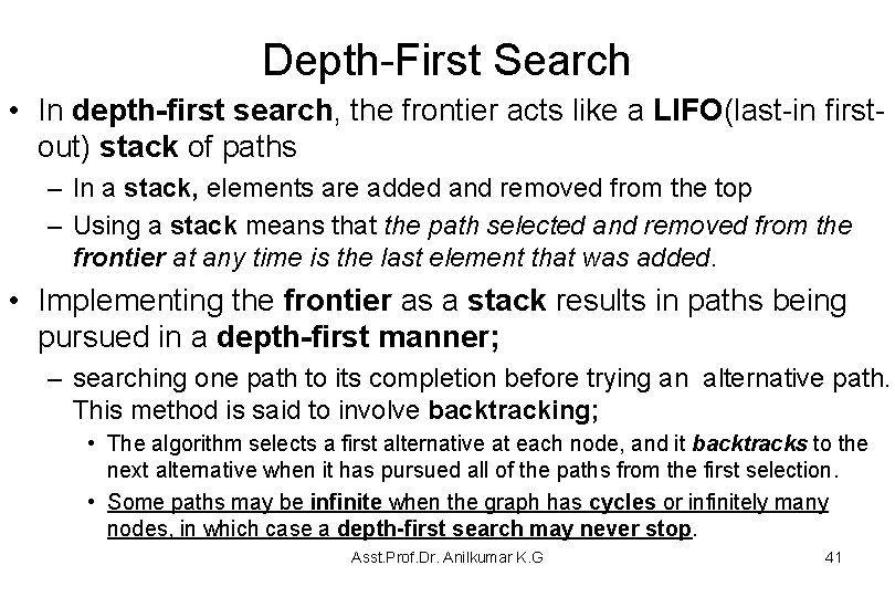
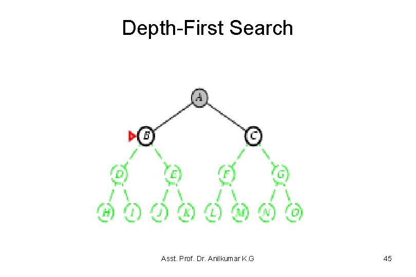
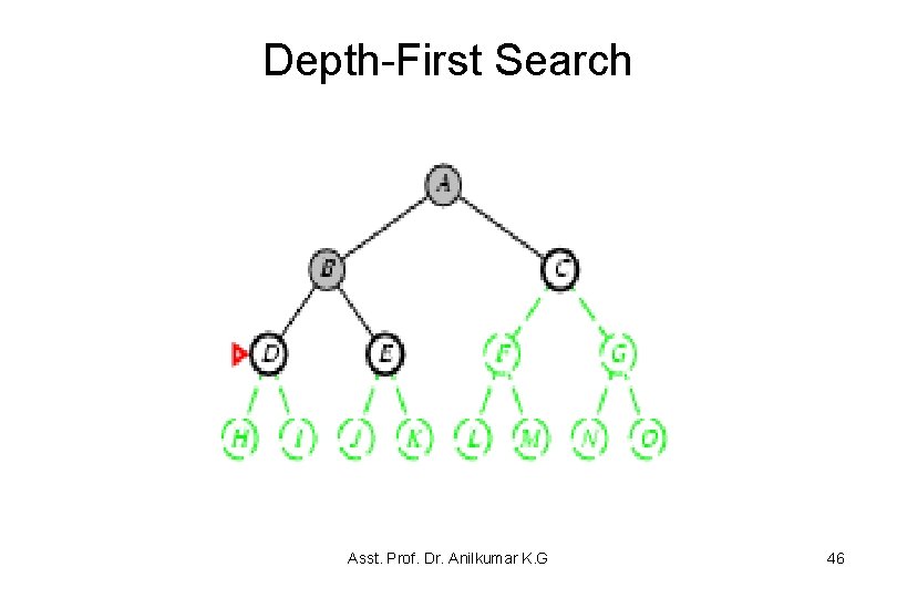
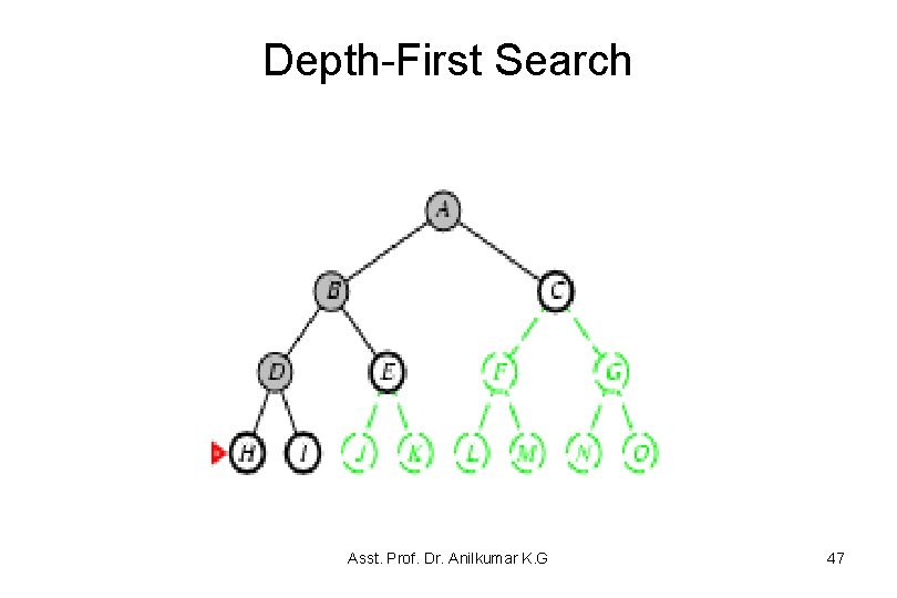
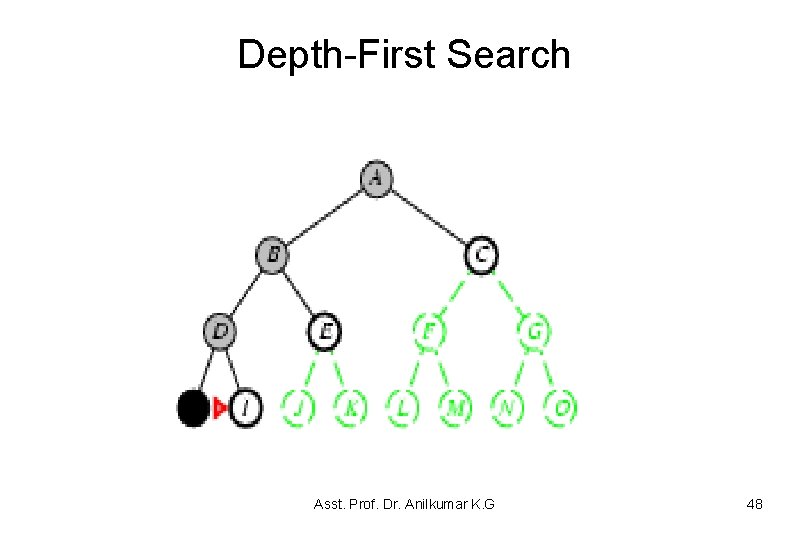
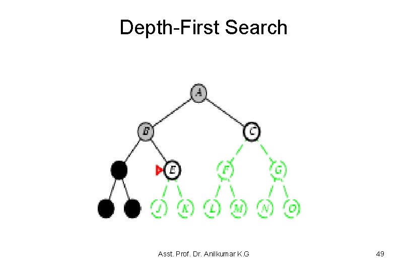
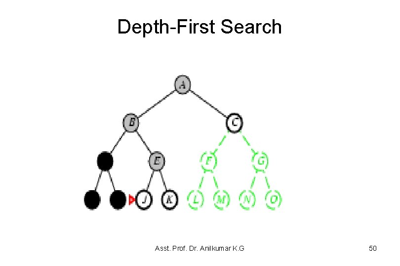
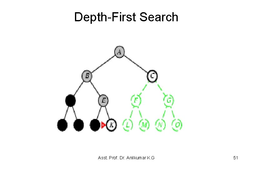
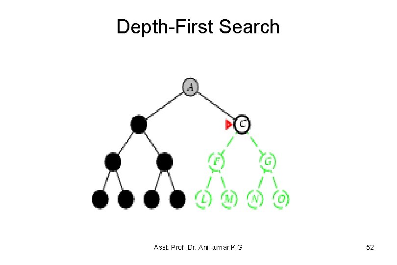
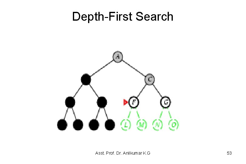
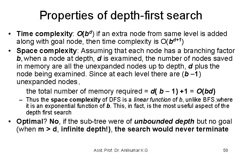
Depth-First Search • In depth-first search, the frontier acts like a LIFO(last-in firstout) stack of paths – In a stack, elements are added and removed from the top – Using a stack means that the path selected and removed from the frontier at any time is the last element that was added. • Implementing the frontier as a stack results in paths being pursued in a depth-first manner; – searching one path to its completion before trying an alternative path. This method is said to involve backtracking; • The algorithm selects a first alternative at each node, and it backtracks to the next alternative when it has pursued all of the paths from the first selection. • Some paths may be infinite when the graph has cycles or infinitely many nodes, in which case a depth-first search may never stop. Asst. Prof. Dr. Anilkumar K. G 41

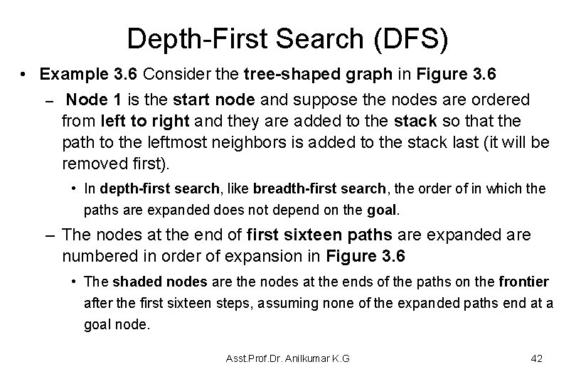
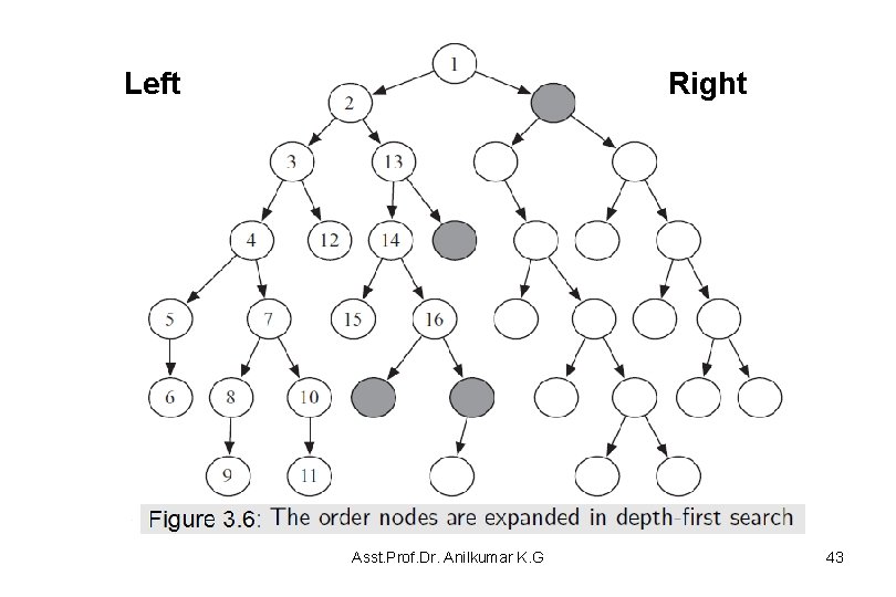
Depth-First Search (DFS) • Example 3. 6 Consider the tree-shaped graph in Figure 3. 6 – Node 1 is the start node and suppose the nodes are ordered from left to right and they are added to the stack so that the path to the leftmost neighbors is added to the stack last (it will be removed first). • In depth-first search, like breadth-first search, the order of in which the paths are expanded does not depend on the goal. – The nodes at the end of first sixteen paths are expanded are numbered in order of expansion in Figure 3. 6 • The shaded nodes are the nodes at the ends of the paths on the frontier after the first sixteen steps, assuming none of the expanded paths end at a goal node. Asst. Prof. Dr. Anilkumar K. G 42

Left Right Asst. Prof. Dr. Anilkumar K. G 43

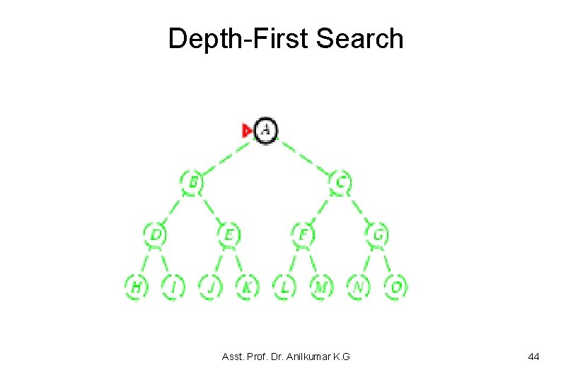
Depth-First Search Asst. Prof. Dr. Anilkumar K. G 44

Depth-First Search Asst. Prof. Dr. Anilkumar K. G 45

Depth-First Search Asst. Prof. Dr. Anilkumar K. G 46

Depth-First Search Asst. Prof. Dr. Anilkumar K. G 47

Depth-First Search Asst. Prof. Dr. Anilkumar K. G 48

Depth-First Search Asst. Prof. Dr. Anilkumar K. G 49

Depth-First Search Asst. Prof. Dr. Anilkumar K. G 50

Depth-First Search Asst. Prof. Dr. Anilkumar K. G 51

Depth-First Search Asst. Prof. Dr. Anilkumar K. G 52

Depth-First Search Asst. Prof. Dr. Anilkumar K. G 53

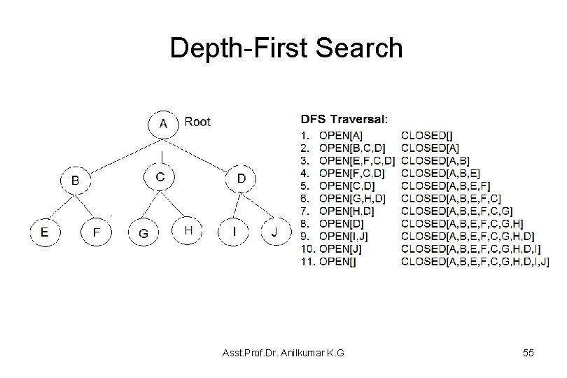
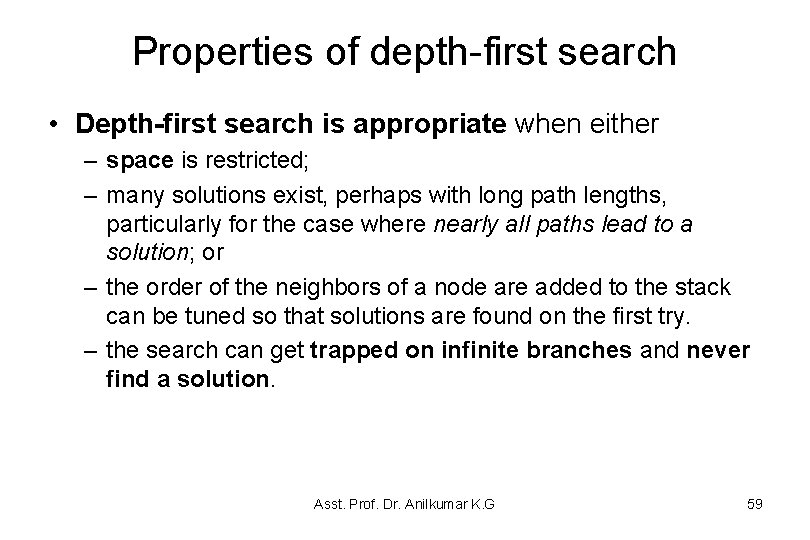
Depth-First Search Procedure List CLOSED, OPEN = [Start Node] //Frontier Loop: If OPEN = NULL, stop // No goal. Else set N = OPEN[0] If N is goal , then stop //Solution Else, remove N from OPEN If N is in CLOSED, then Goto Loop Else, add N to CLOSED Prepend any children of N to OPEN Goto Loop • Here the convention is that nodes are ordered ‘left to right’ Asst. Prof. Dr. Anilkumar K. G 54

Depth-First Search Asst. Prof. Dr. Anilkumar K. G 55

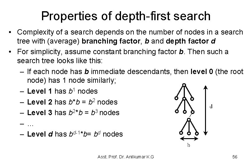
Properties of depth-first search • Complexity of a search depends on the number of nodes in a search tree with (average) branching factor, b and depth factor d • For simplicity, assume constant branching factor b. Then such a search tree looks like this: – If each node has b immediate descendants, then level 0 (the root node) has 1 node similarly; – Level 1 has b 1 nodes – Level 2 has b*b = b 2 nodes – Level 3 has b 2*b = b 3 nodes –… – Level d has bd-1*b= bd nodes Asst. Prof. Dr. Anilkumar K. G 56

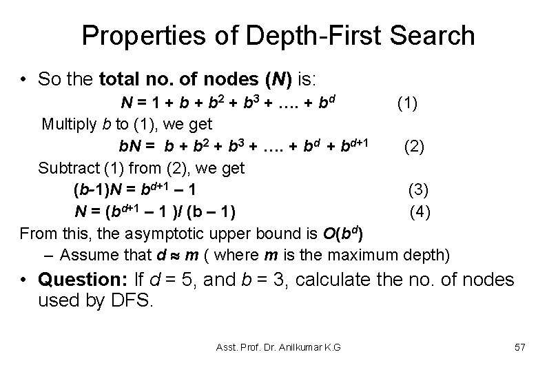
Properties of Depth-First Search • So the total no. of nodes (N) is: N = 1 + b 2 + b 3 + …. + bd (1) Multiply b to (1), we get b. N = b + b 2 + b 3 + …. + bd+1 (2) Subtract (1) from (2), we get (b-1)N = bd+1 – 1 (3) N = (bd+1 – 1 )/ (b – 1) (4) From this, the asymptotic upper bound is O(bd) – Assume that d m ( where m is the maximum depth) • Question: If d = 5, and b = 3, calculate the no. of nodes used by DFS. Asst. Prof. Dr. Anilkumar K. G 57

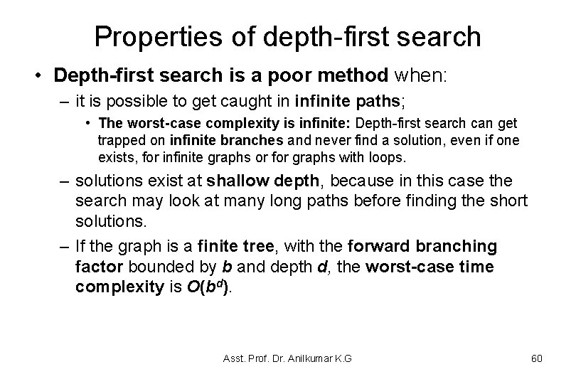
Properties of depth-first search • Time complexity: O(bd) if an extra node from same level is added along with goal node, then time complexity is O(bd+1) • Space complexity: Assuming that each node has a branching factor b, when a node at depth, d is examined, the number of nodes saved in memory are all the unexpanded nodes up to depth, d plus the node being examined. Since at each level there are (b 1) unexpanded nodes , the total number of memory required = d( b 1) +1 = O(bd) – Thus the space complexity of DFS is a linear function of b, unlike BFS , where it is an exponential function of b. This, in fact, is the most useful aspect of the depth first search • Optimal? No, if the sub-tree were of unbounded depth but no goal (when m > d, infinite depth!), the search would never terminate Asst. Prof. Dr. Anilkumar K. G 58

Properties of depth-first search • Depth-first search is appropriate when either – space is restricted; – many solutions exist, perhaps with long path lengths, particularly for the case where nearly all paths lead to a solution; or – the order of the neighbors of a node are added to the stack can be tuned so that solutions are found on the first try. – the search can get trapped on infinite branches and never find a solution. Asst. Prof. Dr. Anilkumar K. G 59

Properties of depth-first search • Depth-first search is a poor method when: – it is possible to get caught in infinite paths; • The worst-case complexity is infinite: Depth-first search can get trapped on infinite branches and never find a solution, even if one exists, for infinite graphs or for graphs with loops. – solutions exist at shallow depth, because in this case the search may look at many long paths before finding the short solutions. – If the graph is a finite tree, with the forward branching factor bounded by b and depth d, the worst-case time complexity is O(bd). Asst. Prof. Dr. Anilkumar K. G 60

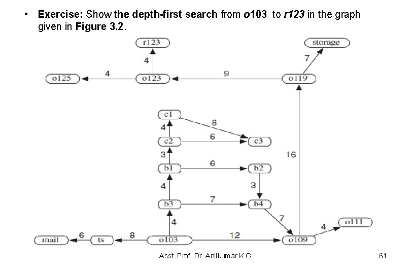
• Exercise: Show the depth-first search from o 103 to r 123 in the graph given in Figure 3. 2. Asst. Prof. Dr. Anilkumar K. G 61

{frontier} = Open[] 1. Open [o 103] Closed[] 2. Open [ts, b 3, o 109] Closed[o 103] 3. Open[mail, b 3, o 109] Closed[o 103, ts] 4. Open[b 3, 0109] Closed[o 103, ts, mail] 5. Open[b 1, b 4, 0109] Closed[o 103, ts, mail, b 3] 6. Open[c 2, b 4, 0109] Closed[0103, ts, mail, b 3, b 1] 7. Open[c 1, c 3, b 2, b 4, 0109] Closed[0103, ts, mail, b 3, b 1, c 2] 8. Open[c 3, b 2, b 4, 0109] Closed[0103, ts, mail, b 3, b 1, c 2, c 1] 9. Open[b 2, b 4, 0109] Closed[0103, ts, mail, b 3, b 1, c 2, c 1, c 3] 10. Open[b 4, 0109] Closed[0103, ts, mail, b 3, b 1, c 2, c 1, c 3, b 2] 11. Open[0109] Closed[0103, ts, mail, b 3, b 1, c 2, c 1, c 3, b 2, b 4] 12. Open[0119, 0111] Closed[0103, ts, mail, b 3, b 1, c 2, c 1, c 3, b 2, b 4, 0109] 13. Open[0123, storage, 0111] Closed[0103, ts, mail, b 3, b 1, c 2, c 1, c 3, b 2, b 4, 0109, 0119] 14. Open[r 123, 0125, storage, 0111] Closed[0103, ts, mail, b 3, b 1, c 2, c 1, c 3, b 2, b 4, 0109, 0119, o 123] 15. Open[0125, storage, 0111] Closed[0103, ts, mail, b 3, b 1, c 2, c 1, c 3, b 2, b 4, 0109, 0119, o 123, r 123] The search has stopped since the goal met. Asst. Prof. Dr. Anilkumar K. G 62

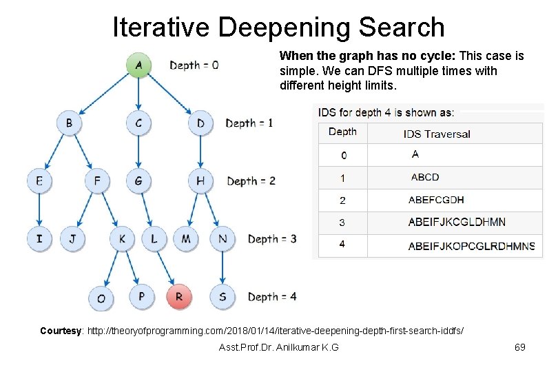
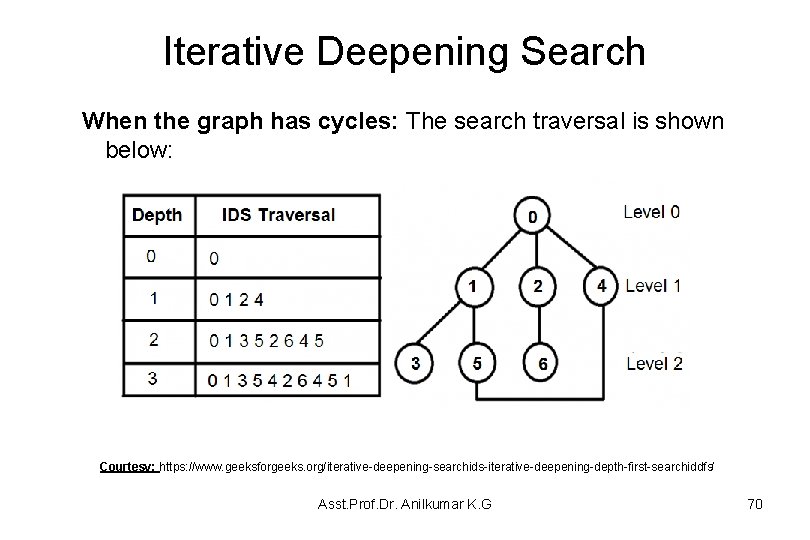
Iterative Deepening Search (IDS) • We have notice that: – Breadth-first search guarantees that a solution path will be found, requires exponential space {O(bd) = O(3 d) when b = 3} – Depth-first search may not halt on infinite graph or graph with cycles. • A hybrid search concept is called an iterative deepening search (IDS) by combining the space efficiency of depth-first search with the optimality of breadth-first search: – The idea is to recompute the elements of the breadth-first frontier rather than storing them – Each recomputation can be a depth-first search which thus uses less space Asst. Prof. Dr. Anilkumar K. G 63

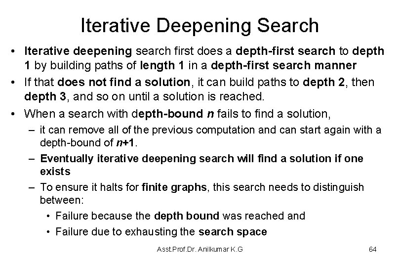
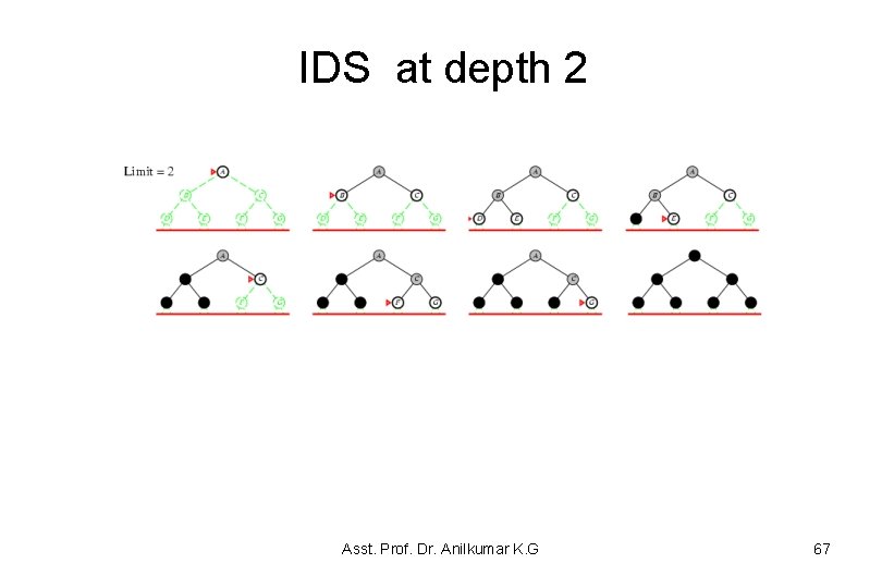
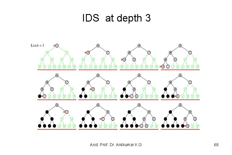
Iterative Deepening Search • Iterative deepening search first does a depth-first search to depth 1 by building paths of length 1 in a depth-first search manner • If that does not find a solution, it can build paths to depth 2, then depth 3, and so on until a solution is reached. • When a search with depth-bound n fails to find a solution, – it can remove all of the previous computation and can start again with a depth-bound of n+1. – Eventually iterative deepening search will find a solution if one exists – To ensure it halts for finite graphs, this search needs to distinguish between: • Failure because the depth bound was reached and • Failure due to exhausting the search space Asst. Prof. Dr. Anilkumar K. G 64

IDS at depth 0 Asst. Prof. Dr. Anilkumar K. G 65

IDS at depth 1 Asst. Prof. Dr. Anilkumar K. G 66

IDS at depth 2 Asst. Prof. Dr. Anilkumar K. G 67

IDS at depth 3 Asst. Prof. Dr. Anilkumar K. G 68

Iterative Deepening Search When the graph has no cycle: This case is simple. We can DFS multiple times with different height limits. Courtesy: http: //theoryofprogramming. com/2018/01/14/iterative-deepening-depth-first-search-iddfs/ Asst. Prof. Dr. Anilkumar K. G 69

Iterative Deepening Search When the graph has cycles: The search traversal is shown below: Courtesy: https: //www. geeksforgeeks. org/iterative-deepening-searchids-iterative-deepening-depth-first-searchiddfs/ Asst. Prof. Dr. Anilkumar K. G 70

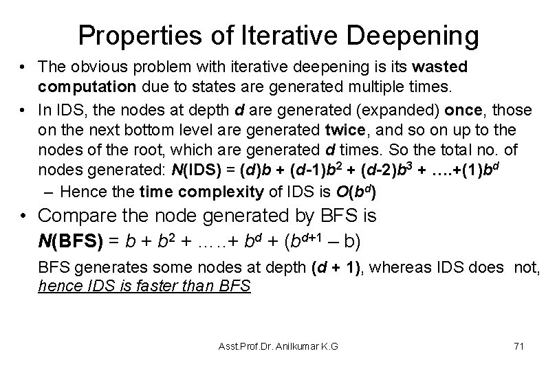
Properties of Iterative Deepening • The obvious problem with iterative deepening is its wasted computation due to states are generated multiple times. • In IDS, the nodes at depth d are generated (expanded) once, those on the next bottom level are generated twice, and so on up to the nodes of the root, which are generated d times. So the total no. of nodes generated: N(IDS) = (d)b + (d-1)b 2 + (d-2)b 3 + …. +(1)bd – Hence the time complexity of IDS is O(bd) • Compare the node generated by BFS is N(BFS) = b + b 2 + …. . + bd + (bd+1 – b) BFS generates some nodes at depth (d + 1), whereas IDS does not, hence IDS is faster than BFS Asst. Prof. Dr. Anilkumar K. G 71

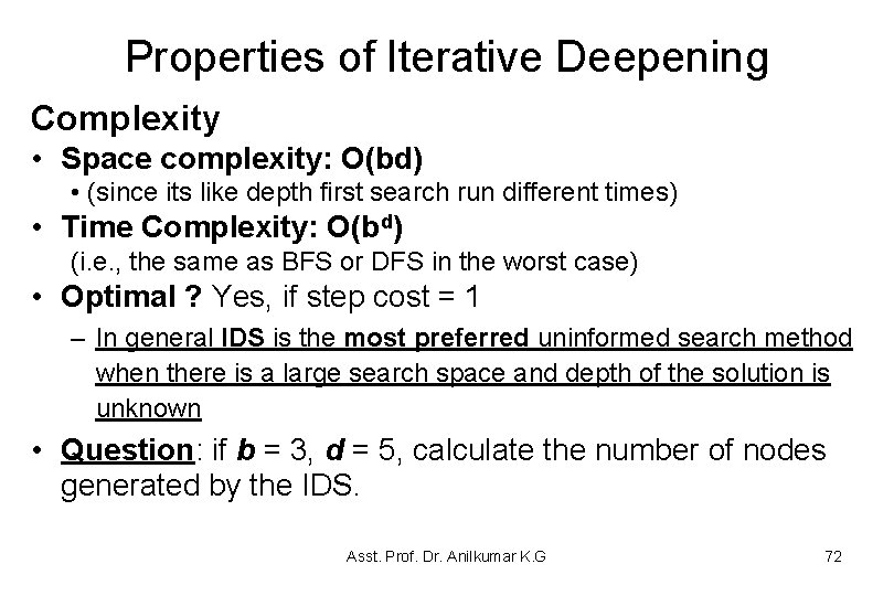
Properties of Iterative Deepening Complexity • Space complexity: O(bd) • (since its like depth first search run different times) • Time Complexity: O(bd) (i. e. , the same as BFS or DFS in the worst case) • Optimal ? Yes, if step cost = 1 – In general IDS is the most preferred uninformed search method when there is a large search space and depth of the solution is unknown • Question: if b = 3, d = 5, calculate the number of nodes generated by the IDS. Asst. Prof. Dr. Anilkumar K. G 72

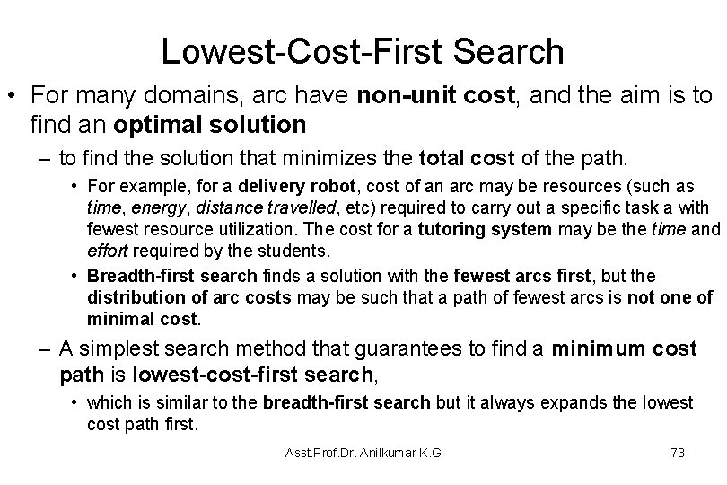
Lowest-Cost-First Search • For many domains, arc have non-unit cost, and the aim is to find an optimal solution – to find the solution that minimizes the total cost of the path. • For example, for a delivery robot, cost of an arc may be resources (such as time, energy, distance travelled, etc) required to carry out a specific task a with fewest resource utilization. The cost for a tutoring system may be the time and effort required by the students. • Breadth-first search finds a solution with the fewest arcs first, but the distribution of arc costs may be such that a path of fewest arcs is not one of minimal cost. – A simplest search method that guarantees to find a minimum cost path is lowest-cost-first search, • which is similar to the breadth-first search but it always expands the lowest cost path first. Asst. Prof. Dr. Anilkumar K. G 73

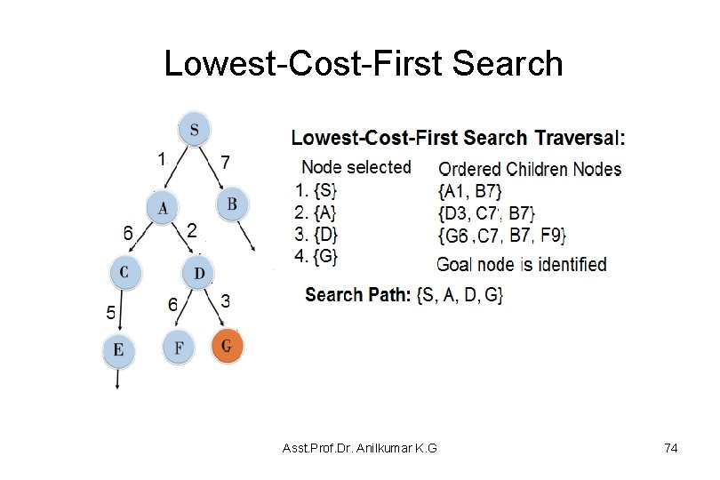
Lowest-Cost-First Search Asst. Prof. Dr. Anilkumar K. G 74

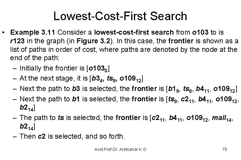
Lowest-Cost-First Search • Example 3. 11 Consider a lowest-cost-first search from o 103 to is r 123 in the graph (in Figure 3. 2). In this case, the frontier is shown as a list of paths in order of cost, where paths are denoted by the node at the end of the path: – Initially the frontier is [o 1030] – At the next stage, it is [b 34, ts 8, o 10912] – Next the path to b 3 is selected, the frontier is [b 18, ts 8, b 411, o 10912] – Next the path to b 1 is selected, the frontier is [ts 8, c 211, b 411, o 10912, b 214] – The path to ts is selected, the frontier is [c 211, b 411, o 10912, mail 14, b 214] – Then c 2 is selected, and so forth. Asst. Prof. Dr. Anilkumar K. G 75

Lowest-Cost-First Search Asst. Prof. Dr. Anilkumar K. G 76

Lowest-Cost-First Search • If the costs of the arcs are bounded below by a positive constant and the branching factor is finite, the lowest-cost-first search is guaranteed to find an optimal solution – a solution with lowest path cost • The lowest-cost-first search expands paths from the start node to goal in the order of their lowest path cost – Such a solution is always optimal • Like breadth-first search, the lowest-cost-first search is typically exponential in both space and time complexities. • It generates all paths from the start that have a cost less than the cost of the solution. Asst. Prof. Dr. Anilkumar K. G 77