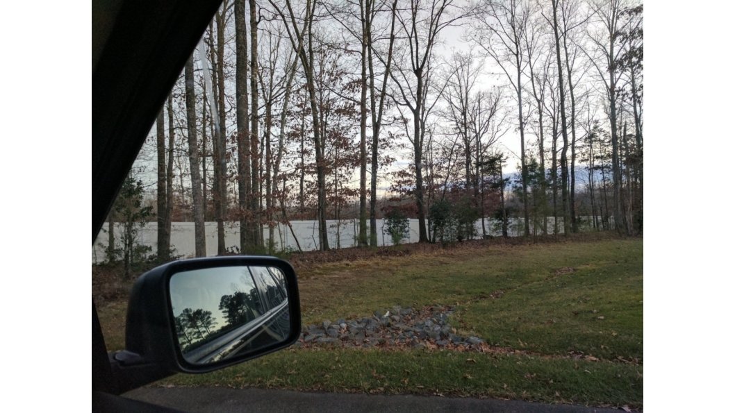
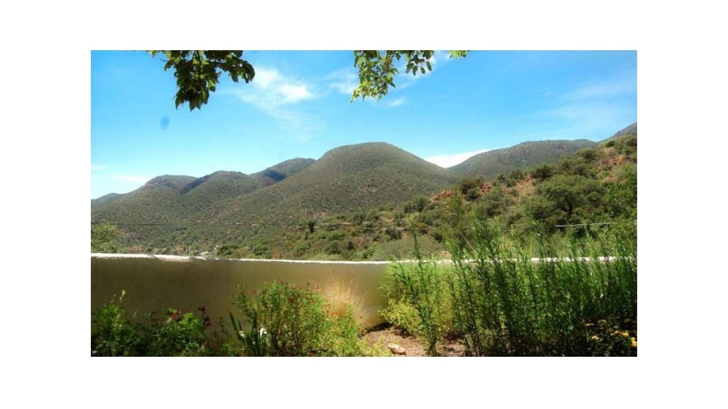
Lets look at some lakefront property actually fences

Let’s look at some lakefront property *actually fences / walls

Recap: Convolutional Network Interpretation 1 Object detectors emerge within CNN trained to classify scenes, without any object supervision!

Recap: Beyond Alex. Net VGG Goog. Le. Net

ave pool, fc 1000 1 x 1 conv, 2048 3 x 3 conv, 512 1 x 1 conv, 2048 3 x 3 conv, 512 1 x 1 conv, 2048 3 x 3 conv, 512 1 x 1 conv, 512, /2 1 x 1 conv, 1024 3 x 3 conv, 256 1 x 1 conv, 256 1 x 1 conv, 1024 3 x 3 conv, 256 1 x 1 conv, 256 1 x 1 conv, 1024 3 x 3 conv, 256 1 x 1 conv, 256 1 x 1 conv, 1024 3 x 3 conv, 256 1 x 1 conv, 256 1 x 1 conv, 1024 3 x 3 conv, 256 1 x 1 conv, 256 1 x 1 conv, 1024 3 x 3 conv, 256 1 x 1 conv, 1024 3 x 3 conv, 256 1 x 1 conv, 256 1 x 1 conv, 1024 3 x 3 conv, 256 1 x 1 conv, 256 1 x 1 conv, 1024 3 x 3 conv, 256 1 x 1 conv, 256 1 x 1 conv, 1024 3 x 3 conv, 256 1 x 1 conv, 1024 3 x 3 conv, 256 1 x 1 conv, 256, /2 1 x 1 conv, 512 3 x 3 conv, 128 1 x 1 conv, 128 1 x 1 conv, 512 3 x 3 conv, 128 1 x 1 conv, 512 3 x 3 conv, 128 1 x 1 conv, 128, /2 1 x 1 conv, 256 3 x 3 conv, 64 1 x 1 conv, 64 7 x 7 conv, 64, /2, pool/2 Deep Residual Learning for Image Recognition Kaiming He, Xiangyu Zhang, Shaoqing Ren, Jian Sun work done at Microsoft Research Asia

Res. Net @ ILSVRC & COCO 2015 Competitions 1 st places in all five main tracks • Image. Net Classification: “Ultra-deep” 152 -layer nets • Image. Net Detection: 16% better than 2 nd • Image. Net Localization: 27% better than 2 nd • COCO Detection: 11% better than 2 nd • COCO Segmentation: 12% better than 2 nd *improvements are relative numbers

Revolution of Depth 28. 2 25. 8 152 layers 16. 4 11. 7 22 layers 6. 7 19 layers 7. 3 3. 57 ILSVRC'15 Res. Net ILSVRC'14 Google. Net ILSVRC'14 VGG 8 layers ILSVRC'13 ILSVRC'12 Alex. Net shallow ILSVRC'11 Image. Net Classification top-5 error (%) ILSVRC'10

101 layers Revolution of Depth Engines of visual recognition 86 58 66 34 16 layers shallow HOG, DPM 8 layers Alex. Net (RCNN) VGG (RCNN) Res. Net (Faster RCNN)* PASCAL VOC 2007 Object Detection m. AP (%) *w/ other improvements & more data

Revolution of Depth Alex. Net, 8 layers (ILSVRC 2012) 11 x 11 conv, 96, /4, pool/2 5 x 5 conv, 256, pool/2 3 x 3 conv, 384 3 x 3 conv, 256, pool/2 fc, 4096 fc, 1000

Revolution of Depth soft max 2 Soft max. Act ivat ion FC Av er age. Pool 7 x 7 + 1 (V) Alex. Net, 8 layers (ILSVRC 2012) 11 x 11 conv, 96, /4, pool/2 5 x 5 conv, 256, pool/2 3 x 3 conv, 384 VGG, 19 layers (ILSVRC 2014) 3 x 3 conv, 64, pool/2 3 x 3 conv, 128 Google. Net, 22 layers (ILSVRC 2014) Dept h. Concat Conv 1 x 1 + 1 (S) 3 x 3 + 1 (S) 5 x 5 + 1 (S) 1 x 1 + 1 (S) Conv Max. Pool 1 x 1 + 1 (S) 3 x 3 + 1 (S) Dept h. Concat Conv 1 x 1 + 1 (S) 3 x 3 + 1 (S) 5 x 5 + 1 (S) soft max 1 1 x 1 + 1 (S) Conv Max. Pool 1 x 1 + 1 (S) 1 x 1 + Soft max. Act ivat ion 1 (S) 3 x 3 + 1 (S) 3 x 3 conv, 384 3 x 3 conv, 128, pool/2 M ax Pool FC 3 x 3 + 2 ( S) Dept h. Concat 3 x 3 conv, 256, pool/2 3 x 3 conv, 256 Conv FC Conv 1 x 1 + 1 (S) 3 x 3 + 1 (S) 5 x 5 + 1 (S) 1 x 1 + 1 (S) Conv Max. Pool Average. Pool 1 x 1 + 1 (S) fc, 4096 3 x 3 + 1 ( S ) 5 x 5 + 3 (V) 3 x 3 conv, 256 Dept h. Concat Conv 1 x 1 + 1 (S) 3 x 3 + 1 (S) 5 x 5 + 1 (S) 1 x 1 + 1 (S) fc, 4096 3 x 3 conv, 256 fc, 1000 3 x 3 conv, 256, pool/2 Conv Max. Pool 1 x 1 + 1 (S) 3 x 3 + 1 (S) Dept h. Concat Conv soft max 0 1 x 1 + 1 (S) 3 x 3 + 1 (S) 5 x 5 + 1 (S) Soft max. Act ivat ion 1 x 1 + 1 (S) Conv Max. Pool 1 x 1 + 1 (S) 1 x 1 + 3 x 3 conv, 512 FC 1 (S) 3 x 3 + 1 (S) Dept h. Concat Conv FC Conv 1 x 1 + 1 (S) 3 x 3 + 1 (S) 5 x 5 + 1 (S) 1 x 1 + 1 (S) 3 x 3 conv, 512 Conv Max. Pool Average. Pool 1 x 1 + 1 (S) 3 x 3 + 1 ( S ) 5 x 5 + 3 (V) Dept h. Concat 3 x 3 conv, 512 Conv 1 x 1 + 1 (S) 3 x 3 + 1 (S) 5 x 5 + 1 (S) 1 x 1 + 1 (S) Conv Max. Pool 1 x 1 + 1 (S) 3 x 3 + 1 (S) 3 x 3 conv, 512, pool/2 M ax Pool 3 x 3 + 2 ( S) Dept h. Concat 3 x 3 conv, 512 Conv 1 x 1 + 1 (S) 3 x 3 + 1 (S) 5 x 5 + 1 (S) 1 x 1 + 1 (S) Conv Max. Pool 1 x 1 + 1 (S) 3 x 3 + 1 (S) 3 x 3 conv, 512 Dept h. Concat Conv 3 x 3 conv, 512 1 x 1 + 1 (S) 3 x 3 + 1 (S) 5 x 5 + 1 (S) 1 x 1 + 1 (S) Conv Max. Pool 1 x 1 + 1 (S) 3 x 3 + 1 (S) M ax Pool 3 x 3 conv, 512, pool/2 3 x 3 + 2 ( S) Local. Resp. Norm Conv fc, 4096 3 x 3 + 1 ( S) Conv 1 x 1 + 1 ( V) Local. Resp. Norm M ax Pool 3 x 3 + 2 ( S) Conv fc, 1000 7 x 7 + 2 ( S) i n pu t

7 x 7 conv, 64, /2, pool/2 1 x 1 conv, 64 3 x 3 conv, 64 1 x 1 conv, 256 1 x 2 conv, 128, /2 Revolution of Depth 3 x 3 conv, 128 1 x 1 conv, 512 1 x 1 conv, 128 3 x 3 conv, 128 1 x 1 conv, 512 1 x 1 conv, 128 3 x 3 conv, 128 1 x 1 conv, 512 1 x 1 conv, 256, /2 3 x 3 conv, 256 1 x 1 conv, 1024 11 x 11 conv, 96, /4, pool/2 Alex. Net, 8 layers (ILSVRC 2012) 5 x 5 conv, 256, pool/2 3 x 3 conv, 384 3 x 3 conv, 256, pool/2 fc, 4096 fc, 1000 VGG, 19 layers (ILSVRC 2014) 3 x 3 conv, 64, pool/2 3 x 3 conv, 128, pool/2 3 x 3 conv, 256, pool/2 3 x 3 conv, 512 3 x 3 conv, 512, pool/2 fc, 4096 fc, 1000 Res. Net, 152 layers (ILSVRC 2015) 1 x 1 conv, 256 3 x 3 conv, 256 1 x 1 conv, 1024 1 x 1 conv, 256 3 x 3 conv, 256 1 x 1 conv, 1024 1 x 1 conv, 256 3 x 3 conv, 256 1 x 1 conv, 1024 1 x 1 conv, 256 3 x 3 conv, 256 1 x 1 conv, 1024 1 x 1 conv, 256 3 x 3 conv, 256 1 x 1 conv, 1024 1 x 1 conv, 256 3 x 3 conv, 256 1 x 1 conv, 1024 1 x 1 conv, 256 3 x 3 conv, 256 1 x 1 conv, 1024 1 x 1 conv, 256 3 x 3 conv, 256 1 x 1 conv, 1024 1 x 1 conv, 256 3 x 3 conv, 256 1 x 1 conv, 1024 1 x 1 conv, 512, /2 3 x 3 conv, 512 1 x 1 conv, 2048 1 x 1 conv, 512 3 x 3 conv, 512 1 x 1 conv, 2048 ave pool, fc 1000

Is learning better networks as simple as stacking more layers?

Simply stacking layers? CIFAR-10 train error (%) test error (%) 20 20 56 -layer 10 10 20 -layer 00 1 2 3 iter. (1 e 4) 4 5 6 0 0 1 2 3 iter. (1 e 4) 4 5 6 • Plain nets: stacking 3 x 3 conv layers… • 56 -layer net has higher training error and test error than 20 -layer net

Simply stacking layers? CIFAR-10 Image. Net-1000 56 -layer 44 -layer 32 -layer 20 -layer 10 5 0 0 plain-20 plain-32 plain-44 plain-56 1 60 50 error (%) 20 34 -layer 40 30 2 3 iter. (1 e 4) 4 5 6 solid: test/val dashed: train 20 0 plain-18 plain-34 10 • “Overly deep” plain nets have higher training error • A general phenomenon, observed in many datasets 18 -layer 20 30 iter. (1 e 4) 40 50

a shallower model (18 layers) 7 x 7 conv, 64, /2 3 x 3 conv, 64 3 x 3 conv, 64 3 x 3 conv, 64 a deeper counterpart (34 layers) 3 x 3 conv, 64 3 x 3 conv, 128, /2 3 x 3 conv, 128 3 x 3 conv, 128 3 x 3 conv, 128 3 x 3 conv, 256, /2 3 x 3 conv, 256 “extra” layers 3 x 3 conv, 256, /2 • A deeper model should not have higher training error 3 x 3 conv, 256 3 x 3 conv, 256 3 x 3 conv, 256 3 x 3 conv, 512, /2 3 x 3 conv, 512 3 x 3 conv, 512 fc 1000 • Richer solution space fc 1000 • A solution by construction: • original layers: copied from a learned shallower model • extra layers: set as identity • at least the same training error • Optimization difficulties: solvers cannot find the solution when going deeper…

Deep Residual Learning �� �� is any desired mapping, • Plain net hope the 2 weight layers fit �� (�� ) �� any two stacked layers weight layer relu weight layer �� (�� ) relu

Deep Residual Learning �� �� is any desired mapping, • Residual net hope the 2 weight layers fit �� (�� ) �� hope the 2 weight layers fit �� (�� ) weight layer �� (�� ) relu weight layer �� �� = �� �� + �� relu identity �� let �� �� = �� �� + ��

Deep Residual Learning • �� �� is a residual mapping w. r. t. identity �� • If identity were optimal, easy to set weights as 0 weight layer �� (�� ) relu weight layer �� �� = �� �� + �� relu identity �� • If optimal mapping is closer to identity, easier to find small fluctuations

Network “Design” • Keep it simple • Our basic design (VGG-style) • all 3 x 3 conv (almost) • spatial size /2 => # filters x 2 • Simple design; just deep! plain net 7 x 7 conv, 64, /2 pool, /2 3 x 3 conv, 64 3 x 3 conv, 64 3 x 3 conv, 64 3 x 3 conv, 128, /2 3 x 3 conv, 128 3 x 3 conv, 128 3 x 3 conv, 128 3 x 3 conv, 128 3 x 3 conv, 256, /2 3 x 3 conv, 256 3 x 3 conv, 256 3 x 3 conv, 256 3 x 3 conv, 256 3 x 3 conv, 256 3 x 3 conv, 256 3 x 3 conv, 512, /2 3 x 3 conv, 512 3 x 3 conv, 512 3 x 3 conv, 512 avg pool fc 1000 Res. Net

CIFAR-10 experiments CIFAR-10 plain nets CIFAR-10 Res. Nets 20 56 -layer 44 -layer 32 -layer 20 -layer 10 5 0 0 plain-20 plain-32 plain-44 plain-56 1 error (%) 20 Res. Net-32 Res. Net-44 Res. Net-56 Res. Net-110 10 5 2 3 iter. (1 e 4) 4 5 6 solid: test dashed: train 0 0 1 2 3 iter. (1 e 4) 4 5 20 -layer 32 -layer 44 -layer 56 -layer 110 -layer 6 • Deep Res. Nets can be trained without difficulties • Deeper Res. Nets have lower training error, and also lower test error

Image. Net experiments Image. Net Res. Nets 60 60 50 50 34 -layer 40 30 20 0 10 20 30 iter. (1 e 4) 18 -layer 40 30 solid: test dashed: train plain-18 plain-34 error (%) Image. Net plain nets 18 -layer 40 50 20 0 Res. Net-18 Res. Net-34 10 34 -layer 20 30 iter. (1 e 4) 40 50 • Deep Res. Nets can be trained without difficulties • Deeper Res. Nets have lower training error, and also lower test error

Image. Net experiments this model has lower time complexity than VGG-16/19 5. 7 • Deeper Res. Nets have lower error 8 7. 4 6. 7 7 6. 1 6 5 4 Res. Net-152 Res. Net-101 Res. Net-50 10 -crop testing, top-5 val error (%) Res. Net-34

Beyond classification A treasure from Image. Net is on learning features. Kaiming He, Xiangyu Zhang, Shaoqing Ren, & Jian Sun. “Deep Residual Learning for Image Recognition”. ar. Xiv 2015.

“Features matter. ” (quote [Girshick et al. 2014], the R-CNN paper) task 2 nd-place winner Res. Nets margin Image. Net Localization (top-5 error) 12. 0 9. 0 27% Image. Net Detection (m. AP@. 5) 16% COCO Detection (m. AP@. 5: . 95) 53. 6 absolute 62. 1 8. 5% better! 33. 5 37. 3 COCO Segmentation (m. AP@. 5: . 95) 25. 1 12% 28. 2 (relative) 11% • Our results are all based on Res. Net-101 • Our features are well transferrable Kaiming He, Xiangyu Zhang, Shaoqing Ren, & Jian Sun. “Deep Residual Learning for Image Recognition”. CVPR 2016.

classifier Object Detection (brief) Ro. I pooling • Simply “Faster R-CNN + Res. Net” Faster R-CNN baseline m. AP@. 5: . 95 VGG-16 41. 5 21. 5 Res. Net-101 48. 4 27. 2 COCO detection results (Res. Net has 28% relative gain) proposals Region Proposal Net feature map CNN image Kaiming He, Xiangyu Zhang, Shaoqing Ren, & Jian Sun. “Deep Residual Learning for Image Recognition”. CVPR 2016. Shaoqing Ren, Kaiming He, Ross Girshick, & Jian Sun. “Faster R-CNN: Towards Real-Time Object Detection with Region Proposal Networks”. NIPS 2015.

Our results on MS COCO *the original image is from the COCO dataset Kaiming He, Xiangyu Zhang, Shaoqing Ren, & Jian Sun. “Deep Residual Learning for Image Recognition”. CVPR 2016. Shaoqing Ren, Kaiming He, Ross Girshick, & Jian Sun. “Faster R-CNN: Towards Real-Time Object Detection with Region Proposal Networks”. NIPS 2015.

Why does Res. Net work so well? • The architecture is somehow easier to optimize. • The authors argue it probably isn’t because it solves the “vanishing gradient” problem.

Opportunities of Scale Computer Vision James Hays Many slides from James Hays, Alyosha Efros, and Derek Hoiem Graphic from Antonio Torralba

Outline Opportunities of Scale: Data-driven methods – The Unreasonable Effectiveness of Data – Scene Completion – Im 2 gps – Recognition via Tiny Images

Computer Vision Class so far • The geometry of image formation – Ancient / Renaissance • Signal processing / Convolution – 1800, but really the 50’s and 60’s • Hand-designed Features for recognition, either instance-level or categorical – 1999 (SIFT), 2003 (Video Google), 2005 (Dalal. Triggs), 2006 (spatial pyramid bag of words) • Learning from Data – 1991 (Eigen. Faces) but late 90’s to now especially

What has changed in the last 15 years? • The Internet • Crowdsourcing • Learning representations from the data these sources provide (deep learning)

Google and massive data-driven algorithms A. I. for the postmodern world: – all questions have already been answered…many times, in many ways – Google is dumb, the “intelligence” is in the data

https: //youtu. be/yv. DCzhbj. YWs? t=24 Watch until 9: 42

Chinese Room, John Searle (1980) If a machine can convincingly simulate an intelligent conversation, does it necessarily understand? In the experiment, Searle imagines himself in a room, acting as a computer by manually executing a program that convincingly simulates the behavior of a native Chinese speaker. Most of the discussion consists of attempts to refute it. "The overwhelming majority, " notes BBS editor Stevan Harnad, “ still think that the Chinese Room Argument is dead wrong. " The sheer volume of the literature that has grown up around it inspired Pat Hayes to quip that the field of cognitive science ought to be redefined as "the ongoing research program of showing Searle's Chinese Room Argument to be false.

Big Idea • Do we need computer vision systems to have strong AI-like reasoning about our world? • What if invariance / generalization isn’t actually the core difficulty of computer vision? • What if we can perform high level reasoning with brute-force, data-driven algorithms?

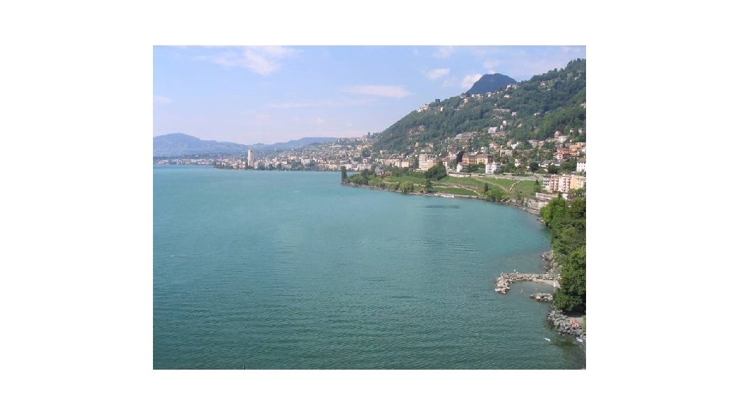
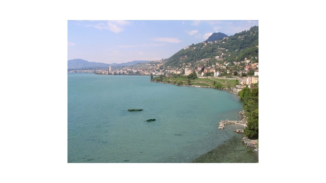
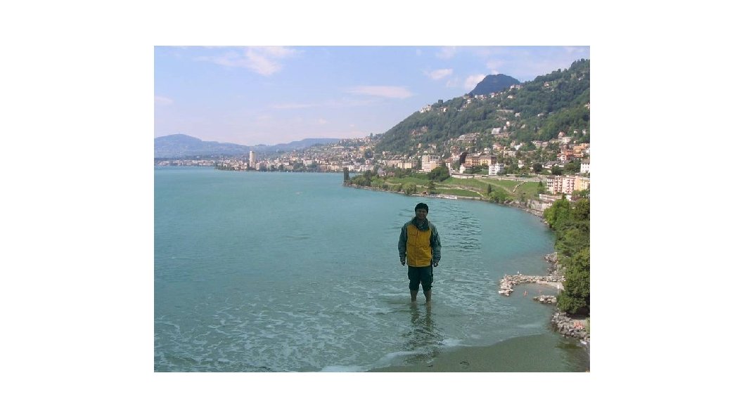
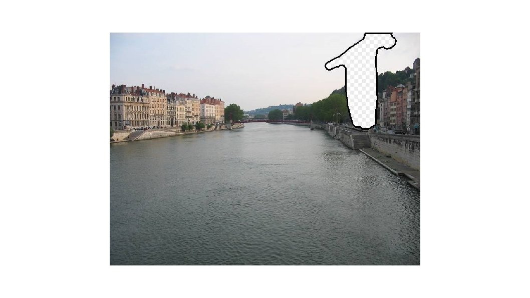
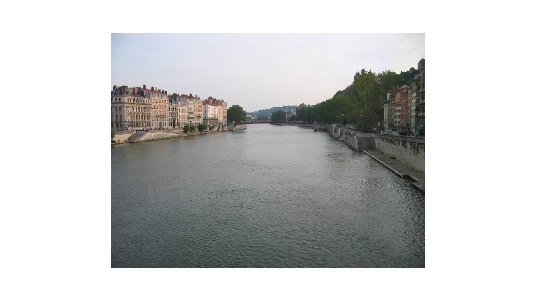
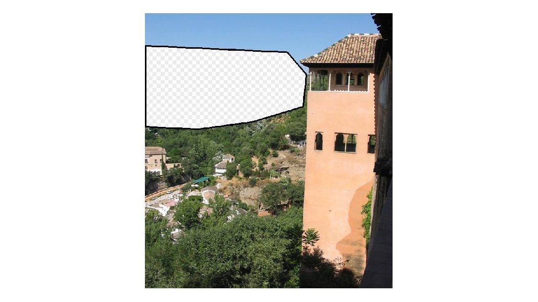
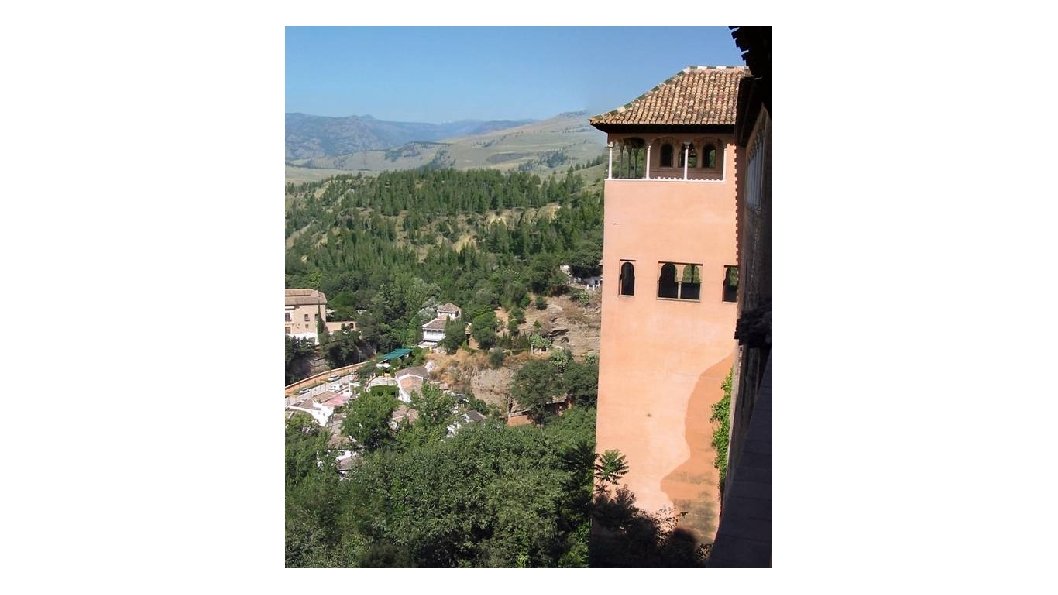
Scene Completion [Hays and Efros. Scene Completion Using Millions of Photographs. SIGGRAPH 2007 and CACM October 2008. ] http: //graphics. cmu. edu/projects/scene-completion/

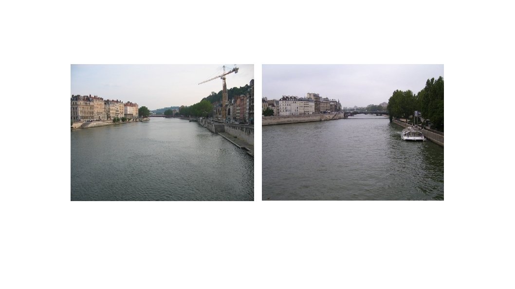
How it works • Find a similar image from a large dataset • Blend a region from that image into the hole Dataset

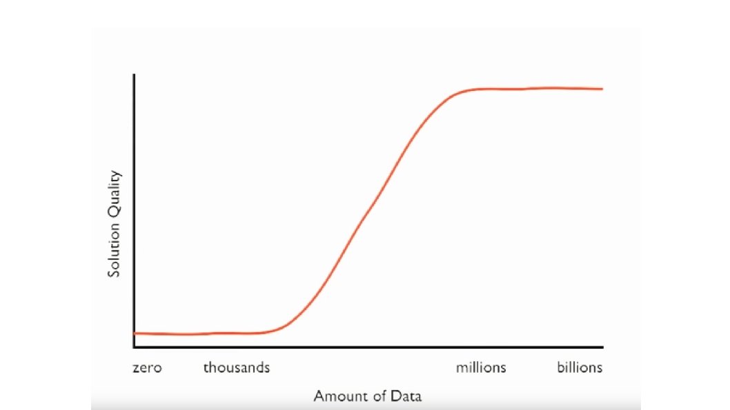
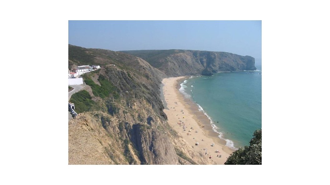
General Principal Huge Dataset Input Images Associated Info image matching Info from Most Similar Images Hopefully, If you have enough images, the dataset will contain very similar images that you can find with simple matching methods.

How many images is enough?

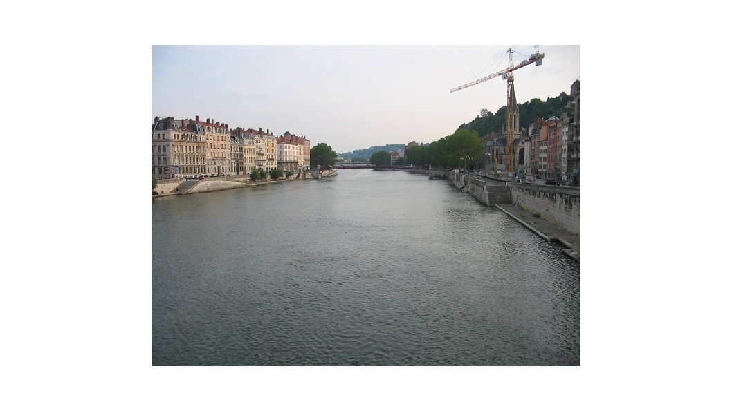
Nearest neighbors from a collection of 20 thousand images

Nearest neighbors from a collection of 2 million images

Image Data on the Internet • Flickr (as of Sept. 19 th, 2010) – 5 billion photographs – 100+ million geotagged images • Facebook (as of 2009) – 15 billion http: //royal. pingdom. com/2010/01/22/internet-2009 -in-numbers/

Image Data on the Internet • Flickr (as of Nov 2013) – 10 billion photographs – 100+ million geotagged images – 3. 5 million a day • Facebook (as of Sept 2013) – 250 billion+ – 300 million a day • Instagram – 55 million a day

Scene Completion: how it works [Hays and Efros. Scene Completion Using Millions of Photographs. SIGGRAPH 2007 and CACM October 2008. ]

The Algorithm

Scene Matching

Scene Descriptor

Scene Descriptor Scene Gist Descriptor (Oliva and Torralba 2001)

Scene Descriptor + Scene Gist Descriptor (Oliva and Torralba 2001)

2 Million Flickr Images

… 200 total

Context Matching

Graph cut + Poisson blending

Result Ranking We assign each of the 200 results a score which is the sum of: The scene matching distance The context matching distance (color + texture) The graph cut cost

… 200 scene matches

Which is the original?

To be continued