Lecture 5 Model Evaluation Elements of Model evaluation

Lecture 5 Model Evaluation

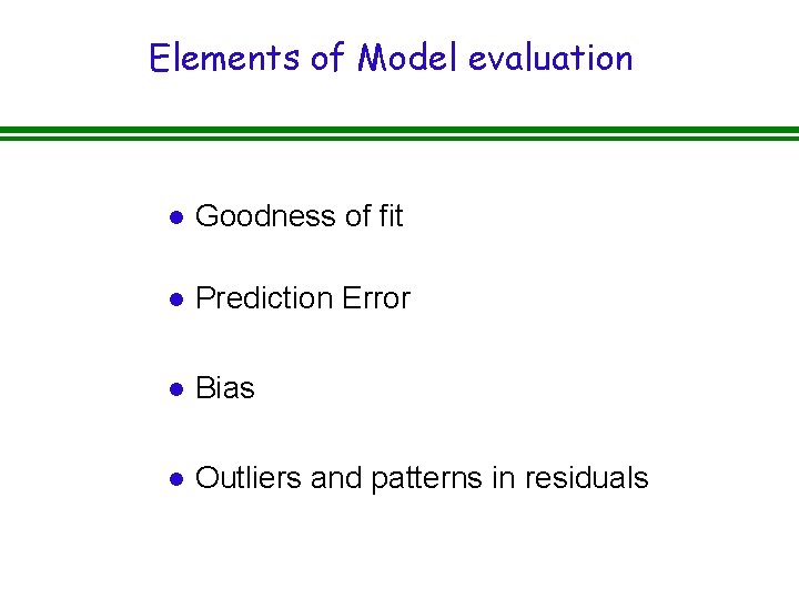
Elements of Model evaluation l Goodness of fit l Prediction Error l Bias l Outliers and patterns in residuals

Assessing Goodness of Fit for Continuous Data l Visual methods - Don’t underestimate the power of your eyes, but eyes can deceive, too. . . l Quantification - A variety of traditional measures, all with some limitations. . . A good review. . . C. D. Schunn and D. Wallach. Evaluating Goodness-of-Fit in Comparison of Models to Data. Source: http: //www. lrdc. pitt. edu/schunn/gof/GOF. doc

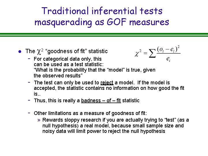
Traditional inferential tests masquerading as GOF measures l The c 2 “goodness of fit” statistic - For categorical data only, this can be used as a test statistic: “What is the probability that the “model” is true, given the observed results” The test can only be used to reject a model. If the model is accepted, the statistic contains no information on how good the fit is. . Thus, this is really a badness – of – fit statistic Other limitations as a measure of goodness of fit: » Rewards sloppy research if you are actually trying to “test” (as a null hypothesis) a real model, because small sample size and noisy data will limit power to reject the null hypothesis

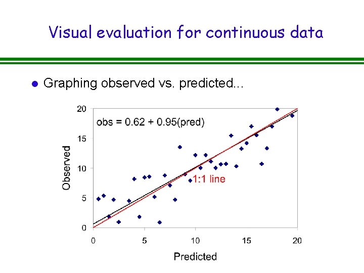
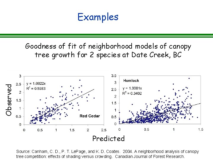
Visual evaluation for continuous data l Graphing observed vs. predicted. . .

Examples Observed Goodness of fit of neighborhood models of canopy tree growth for 2 species at Date Creek, BC Predicted Source: Canham, C. D. , P. T. Le. Page, and K. D. Coates. 2004. A neighborhood analysis of canopy tree competition: effects of shading versus crowding. Canadian Journal of Forest Research.

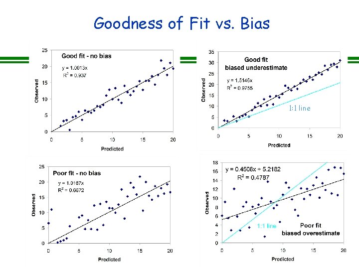
Goodness of Fit vs. Bias 1: 1 line

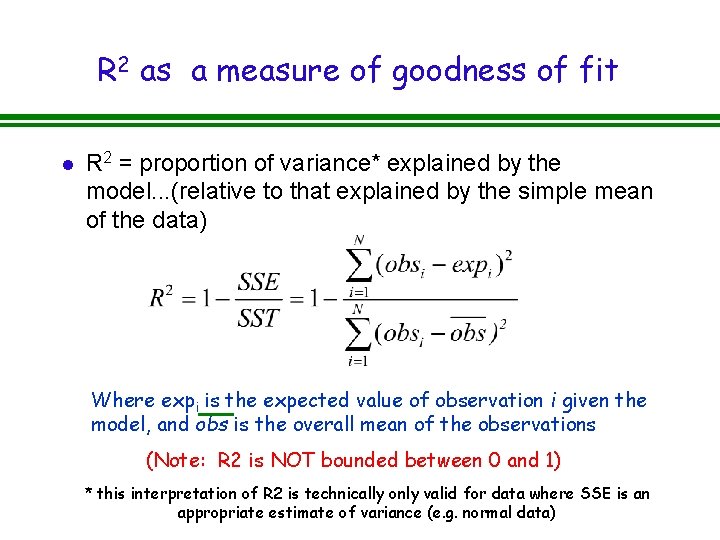
R 2 as a measure of goodness of fit l R 2 = proportion of variance* explained by the model. . . (relative to that explained by the simple mean of the data) Where expi is the expected value of observation i given the model, and obs is the overall mean of the observations (Note: R 2 is NOT bounded between 0 and 1) * this interpretation of R 2 is technically only valid for data where SSE is an appropriate estimate of variance (e. g. normal data)

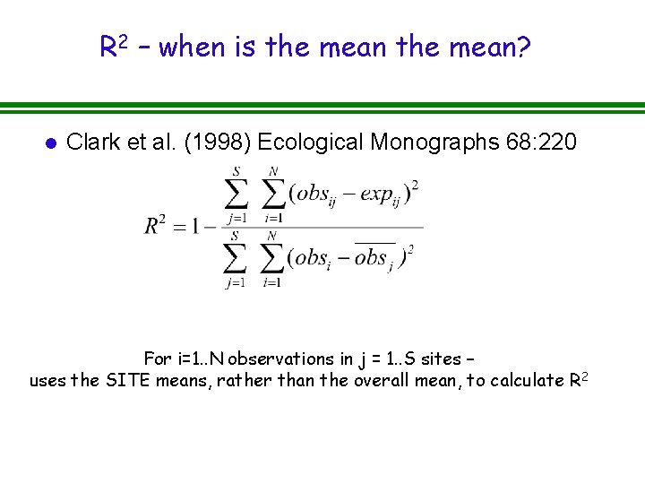
R 2 – when is the mean? l Clark et al. (1998) Ecological Monographs 68: 220 For i=1. . N observations in j = 1. . S sites – uses the SITE means, rather than the overall mean, to calculate R 2

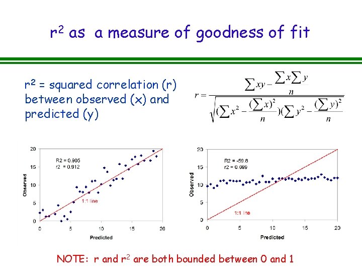
r 2 as a measure of goodness of fit r 2 = squared correlation (r) between observed (x) and predicted (y) NOTE: r and r 2 are both bounded between 0 and 1

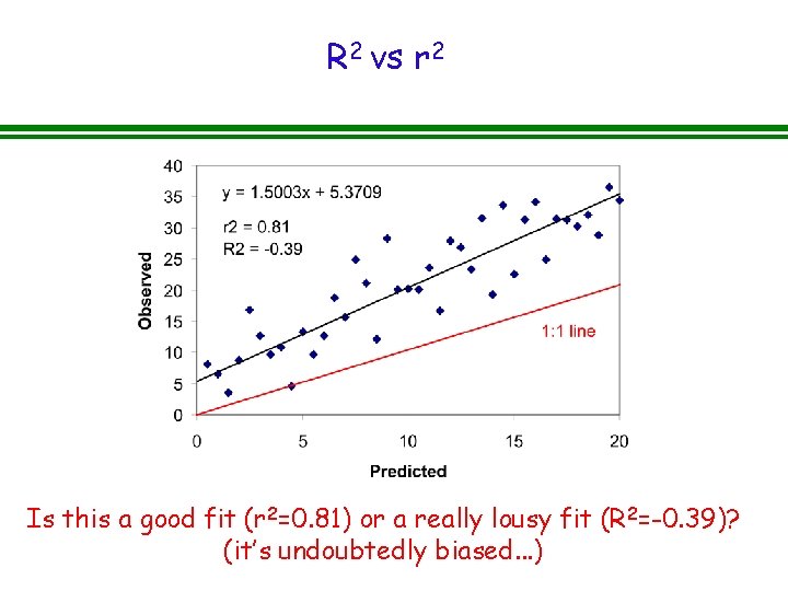
R 2 vs r 2 Is this a good fit (r 2=0. 81) or a really lousy fit (R 2=-0. 39)? (it’s undoubtedly biased. . . )

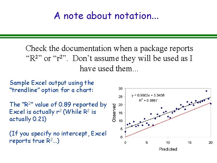
A note about notation. . . Check the documentation when a package reports “R 2” or “r 2”. Don’t assume they will be used as I have used them. . . Sample Excel output using the “trendline” option for a chart: The “R 2” value of 0. 89 reported by Excel is actually r 2 (While R 2 is actually 0. 21) (If you specify no intercept, Excel reports true R 2. . . )

R 2 vs. r 2 for goodness of fit l When there is no bias, the two measures will be almost identical (but I prefer R 2, in principle). l When there is bias, R 2 will be low to negative, but r 2 will indicate how good the fit could be after taking the bias into account. . .

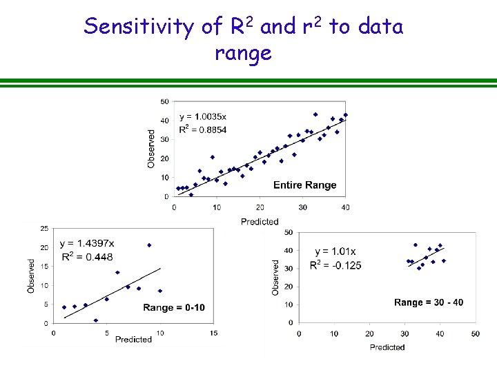
Sensitivity of R 2 and r 2 to data range

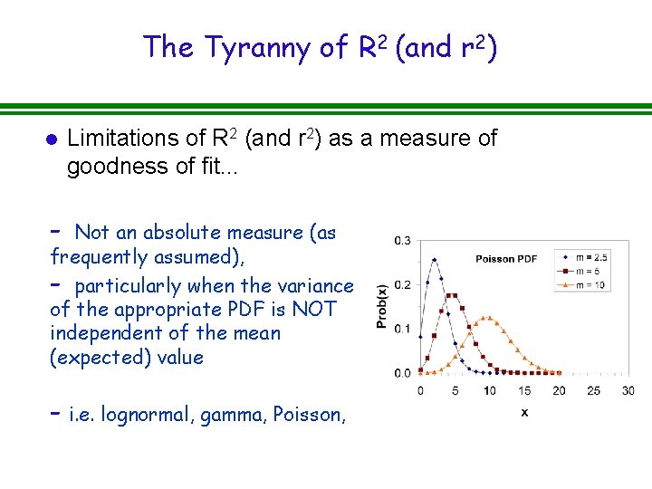
The Tyranny of R 2 (and r 2) l Limitations of R 2 (and r 2) as a measure of goodness of fit. . . - Not an absolute measure (as frequently assumed), - particularly when the variance of the appropriate PDF is NOT independent of the mean (expected) value - i. e. lognormal, gamma, Poisson,

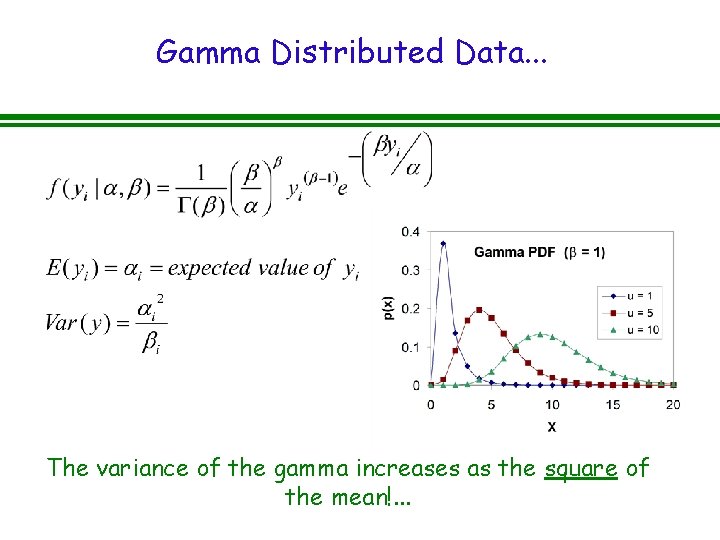
Gamma Distributed Data. . . The variance of the gamma increases as the square of the mean!. . .

So, how good is good? l Our assessment is ALWAYS subjective, because of - Complexity of the process being studied - Sources of noise in the data l From a likelihood perspective, should you ever expect R 2 = 1?

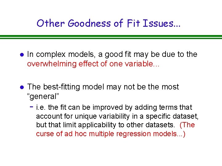
Other Goodness of Fit Issues. . . l In complex models, a good fit may be due to the overwhelming effect of one variable. . . l The best-fitting model may not be the most “general” - i. e. the fit can be improved by adding terms that account for unique variability in a specific dataset, but that limit applicability to other datasets. (The curse of ad hoc multiple regression models. . . )

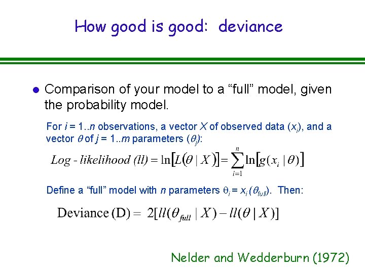
How good is good: deviance l Comparison of your model to a “full” model, given the probability model. For i = 1. . n observations, a vector X of observed data (xi), and a vector q of j = 1. . m parameters (qj): Define a “full” model with n parameters qi = xi (qfull). Then: Nelder and Wedderburn (1972)

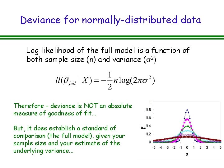
Deviance for normally-distributed data Log-likelihood of the full model is a function of both sample size (n) and variance (s 2) Therefore – deviance is NOT an absolute measure of goodness of fit. . . But, it does establish a standard of comparison (the full model), given your sample size and your estimate of the underlying variance. . .

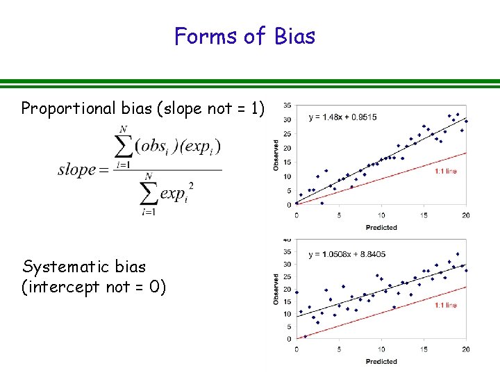
Forms of Bias Proportional bias (slope not = 1) Systematic bias (intercept not = 0)

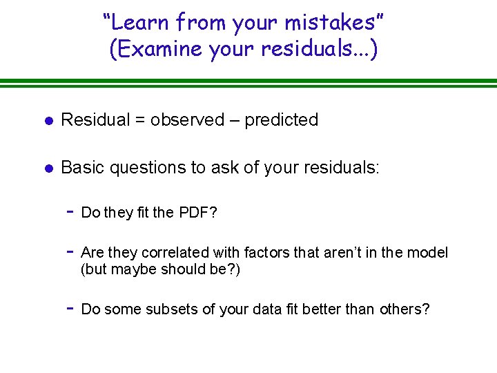
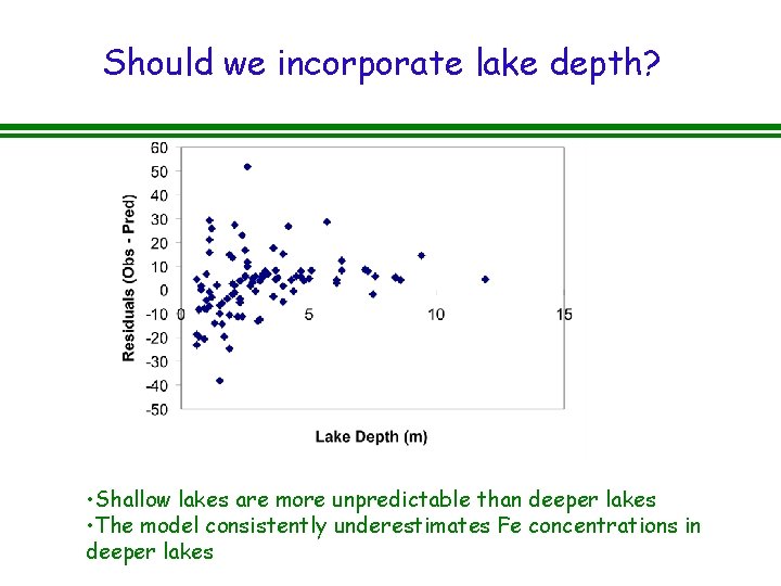
“Learn from your mistakes” (Examine your residuals. . . ) l Residual = observed – predicted l Basic questions to ask of your residuals: - Do they fit the PDF? - Are they correlated with factors that aren’t in the model (but maybe should be? ) - Do some subsets of your data fit better than others?

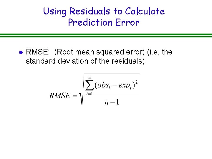
Using Residuals to Calculate Prediction Error l RMSE: (Root mean squared error) (i. e. the standard deviation of the residuals)

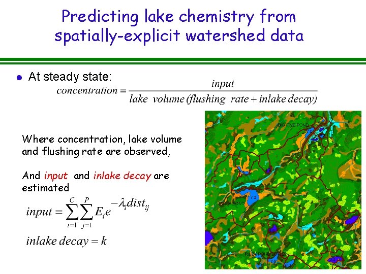
Predicting lake chemistry from spatially-explicit watershed data l At steady state: Where concentration, lake volume and flushing rate are observed, And input and inlake decay are estimated

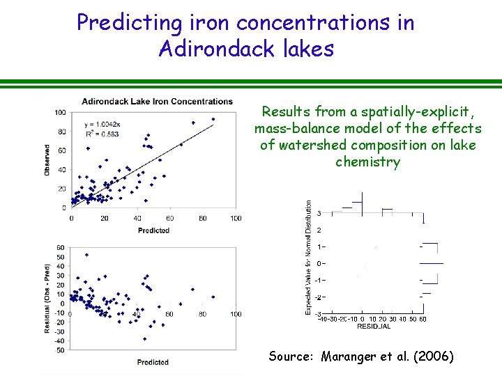
Predicting iron concentrations in Adirondack lakes Results from a spatially-explicit, mass-balance model of the effects of watershed composition on lake chemistry Source: Maranger et al. (2006)

Should we incorporate lake depth? • Shallow lakes are more unpredictable than deeper lakes • The model consistently underestimates Fe concentrations in deeper lakes

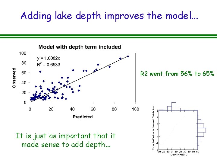
Adding lake depth improves the model. . . R 2 went from 56% to 65% It is just as important that it made sense to add depth. . .

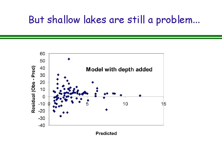
But shallow lakes are still a problem. . .

Summary – Model Evaluation l There are no silver bullets. . . l The issues are even muddier for categorical data. . . l An increase in goodness of fit does not necessarily result in an increase in knowledge… - Increasing goodness of fit reduces uncertainty in the - predictions of the models, but this costs money (more and better data). How much are you willing to spend? The “signal to noise” issue: if you can see the signal