LECTURE 22 VAR 1 Methods of calculating VAR

LECTURE 22 VAR 1

Methods of calculating VAR (Cont. ) • Correlation method is conceptually simple and easy to apply; it only requires the mean returns and the covariance matrix of asset returns. • 2) Historical Simulation: Historical simulation uses actual historic data to predict the returns of risk factors instead of assuming risk factor returns have a normal distribution. • • To use this simulation to estimate VAR, a risk manager must follow these steps: • Gather the market data for each of the assets over the historical period. Value-At-Risk 2

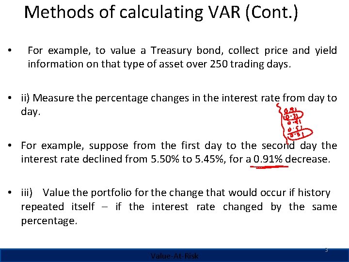
Methods of calculating VAR (Cont. ) • For example, to value a Treasury bond, collect price and yield information on that type of asset over 250 trading days. • ii) Measure the percentage changes in the interest rate from day to day. • For example, suppose from the first day to the second day the interest rate declined from 5. 50% to 5. 45%, for a 0. 91% decrease. • iii) Value the portfolio for the change that would occur if history repeated itself – if the interest rate changed by the same percentage. Value-At-Risk 3

Methods of calculating VAR (Cont. ) • For the first sample path in the simulation, decrease the interest rate by 0. 91%, for example from 6. 00% to 5. 94%. Then the bond is valued with this interest rate to calculate a future value. • By subtracting the future portfolio value from the current value, an analyst can know the amount that would be lost due to market risk if these conditions occurred again. • Repeat this analysis for each trading day in the data period, creating a distribution of possible outcomes for the portfolio. Value-At-Risk 4

Methods of calculating VAR (Cont. ) • When the distribution is complete, rank all the possible outcomes by gain (or loss) and choose a confidence level for the estimate. • The value at that percentile in the distribution represents the VAR for that portfolio. • In a simulation of 100 historical trading days, to estimate VAR to the 95% confidence level, select the fifth worst value in the distribution. • If the historical period is 1000 days, select the fiftieth worst value, and so on. In this way, different confidence levels can be achieved. Value-At-Risk 5

Methods of calculating VAR (Cont. ) 3) Monte Carlo Simulation: is much more comprehensive and rigorous than historical simulation because it takes greater account of the potential for market shocks and uses mathematical modeling to predict future shocks. • To use this simulation method to estimate VAR, a risk manager must do the following: i. Use the past changes of risk factors such as interest rates for the historical period to generate an equation to model these changes. • This model is usually generated through some regression analysis. Value-At-Risk form of 6

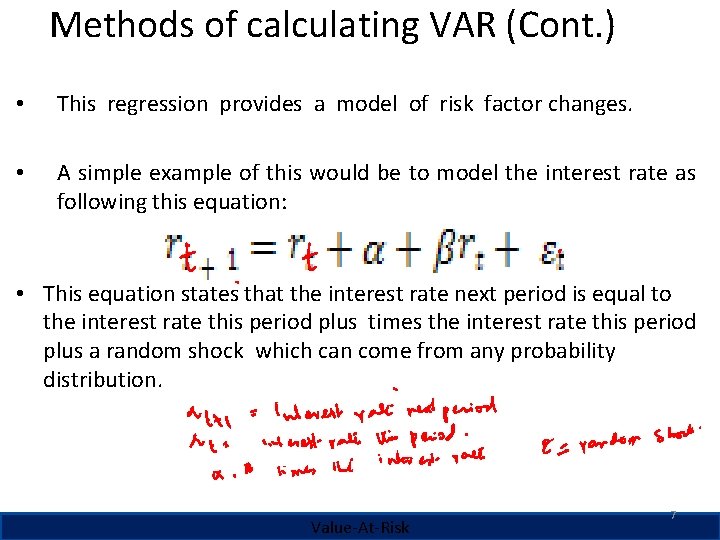
Methods of calculating VAR (Cont. ) • This regression provides a model of risk factor changes. • A simple example of this would be to model the interest rate as following this equation: • This equation states that the interest rate next period is equal to the interest rate this period plus times the interest rate this period plus a random shock which can come from any probability distribution. Value-At-Risk 7

Methods of calculating VAR (Cont. ) • Using actual data this equation can be estimated to get the values of these regression parameters and the variance of the random shock. • Armed with these parameters, a range of future outcomes can be generated for the future interest rate by generating random numbers for. ii) Simulate the behavior of the risk factors in the next period. • Given current values and a distribution of random numbers which predicts future values, the model should calculate a possible future value for a risk factor. Value-At-Risk 8

Methods of calculating VAR (Cont. ) • When this simulation is repeated a large number of times (for example, at least 10, 000), it forms a distribution of possible future values. • Each of these values has a probability of occurring assigned to it, based on the random distribution used to generate the distribution. • Like the historical simulation, the portfolio values can be ranked from lowest to highest, along with their corresponding probability of occurring. • The risk manager chooses a level of significance for the VAR estimate, for example 5%. When the cumulative probability of the distribution reaches 5%, the corresponding future value is the VAR estimate. Value-At-Risk 9

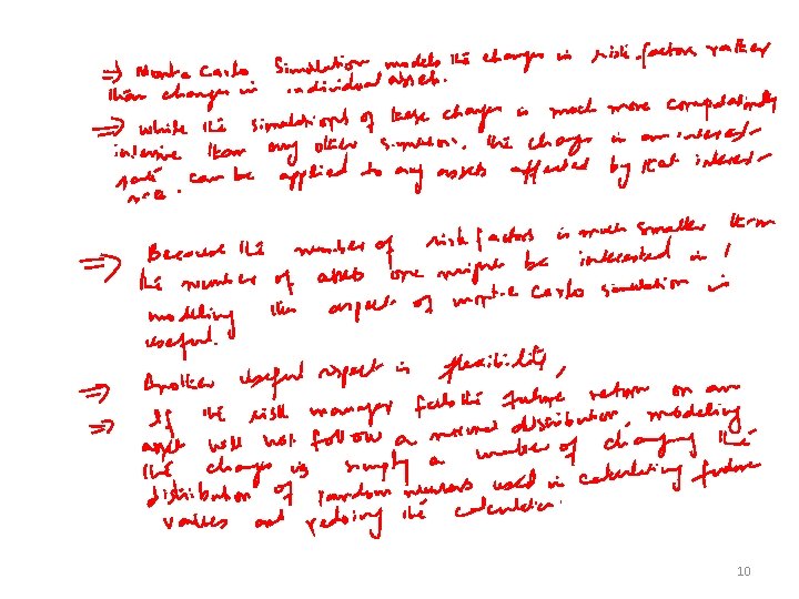
10

Critique of VAR • The Correlation Model is the least complex, mainly because it makes some simplifying assumptions: normality of returns and constant correlations between risk factors. • Therefore it is one of the fastest and easiest reports to generate. • The Historical Simulation Model is more complicated, as it uses exact trends in historical prices to allow for the greater presence of shocks to the market. • However, it assumes past prices are a good predictor of future prices and only uses a single sample path of prices to compute VAR, which might not reliably reflect the future. Value-At-Risk 11

Critique of VAR (Cont. ) • Monte Carlo Simulation is the most complicated of the three, but it is also the most flexible, as it incorporates historical data with statistical constraints set by the risk manager in a mathematical model over many sample paths. • However, because of its tremendous complexity, it is also considerably more difficult and time consuming to calculate; considering the purpose of VAR – to arrive at a simple calculation for changes in a firm’s value – this effort may be too much for some firms. Value-At-Risk 12

Worst Case Scenario Analysis • Part of the problem some risk managers have with VAR is that it is only a probabilistic measure of what will happen to a portfolio. • If a risk manager uses a 95% confidence level for VAR, then on average once every 20 trading days (about once a month) the loss will exceed the estimate. Statistically, the loss will be greater than 1. 65 standard deviations from the mean loss once every 20 periods. • Even if a risk manager uses a 99% confidence level, the estimate will still be wrong once every 100 trading days (roughly once every five months), with a loss greater than 2. 33 standard deviations every 100 periods. Value-At-Risk 13

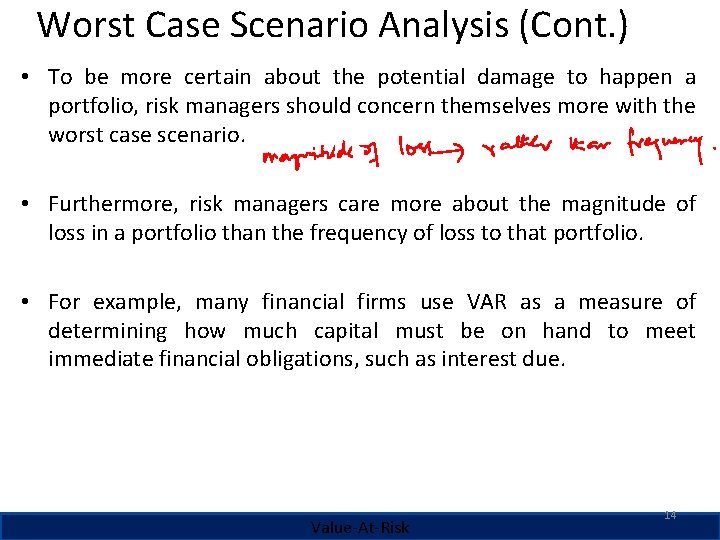
Worst Case Scenario Analysis (Cont. ) • To be more certain about the potential damage to happen a portfolio, risk managers should concern themselves more with the worst case scenario. • Furthermore, risk managers care more about the magnitude of loss in a portfolio than the frequency of loss to that portfolio. • For example, many financial firms use VAR as a measure of determining how much capital must be on hand to meet immediate financial obligations, such as interest due. Value-At-Risk 14

Worst Case Scenario Analysis (Cont. ) • Suppose a bank needs to know how much capital it must have to meet interest payments. • While it would be upset to lose money any day, as long as it holds enough capital to meet its financial obligations, it will survive. • However, if the bank grossly underestimates its capital requirements, and as a result of a loss from market risk, it is unable to make interest payments, it will default on its interest payments and destroy the bank. • In this case, the risk managers cannot afford to underestimate the VAR even once. Value-At-Risk 15

Worst Case Scenario Analysis (Cont. ) • A simple way some risk managers deal with this threat is to multiply the VAR value by some number of their own choosing, such as three. • The regulators at the BASLE in Europe have adopted this very same ad hoc approach to worst case risk management. • If a risk manager was using the 1% level of VAR (2. 33 standard deviations), and multiplied it by 3 to calculate capital requirements, the firm should be safe for a loss up to seven standard deviations (3*2. 33=7), which is extremely unlikely. Value-At-Risk 16

Worst Case Scenario Analysis (Cont. ) • This measure may be effective, but it is imprecise and inefficient. In an effort to arrive at a more precise number to measure capital requirements, financial analysts have applied stress testing to their VAR models to study the worst case scenario. • Worst case scenario analysis is a complementary measure to VAR. • The basic premise is that by estimating VAR a large number of times, a risk manager can create a distribution of worst case scenario outcomes, and from that distribution compute the worst case scenario for the portfolio. Value-At-Risk 17

Worst Case Scenario Analysis (Cont. ) • Suppose a risk manager uses Monte Carlo simulation to measure VAR. Worst case scenario analysis consists of the following steps: • Choose the period over which to measure the worst case. • Usually this is a short term period, such as a week, month, or quarter, although some risk managers might study the worst case over an entire year. • ii. (at least 10, 000). Each simulation represents the behavior of a portfolio over the trading days in the chosen period of time. Value-At-Risk 18

Worst Case Scenario Analysis (Cont. ) • This analysis assumes traders manage their portfolios actively to maintain constant levels of variance, rather than holding the same assets over time. • As a result, each path in a Monte Carlo simulation relies on the original portfolio weights, as they are constant over time. • This is called homogenous analysis. (If the parameters for each market factor in the analysis, i. e. mean and variance, etc. were allowed to vary over time, this method would be classified as nonhomogenous analysis. ) Value-At-Risk 19

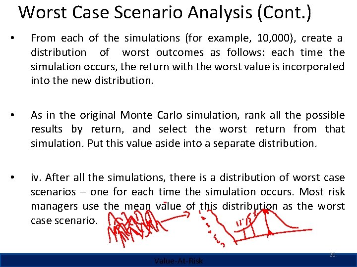
Worst Case Scenario Analysis (Cont. ) • From each of the simulations (for example, 10, 000), create a distribution of worst outcomes as follows: each time the simulation occurs, the return with the worst value is incorporated into the new distribution. • As in the original Monte Carlo simulation, rank all the possible results by return, and select the worst return from that simulation. Put this value aside into a separate distribution. • iv. After all the simulations, there is a distribution of worst case scenarios – one for each time the simulation occurs. Most risk managers use the mean value of this distribution as the worst case scenario. Value-At-Risk 20

Worst Case Scenario Analysis (Cont. ) • To be even more risk-averse, sometimes risk managers want to know the values of the distribution at the 5% or 1% levels, which can easily be taken from the distribution as well. • Example: Suppose an analyst makes a worst case scenario analysis for a portfolio with a mean return of 0 and a return volatility of 1. • The following table summarizes the worst case scenario values. Value-At-Risk 21

Thanks For being Patient…. 22