Islamic University of Gaza Faculty of Engineering Electrical

Islamic University of Gaza Faculty of Engineering Electrical Engineering Department CH 10: ØFrequency Response Techniques Control Systems Design, Dr. Moayed Almobaied

Frequency Response Frequency response methods, developed by Nyquist and Bode in the 1930 s, are older than the root locus method, which was discovered by Evans in 1948 (Nyquist, 1932; Bode, 1945). The older method, is not as intuitive as the root locus. However, frequency response yields a new vantage point from which to view feedback control systems. This technique has distinct advantages in the following situations: 1. When modeling transfer functions from physical data. 2. When designing lead compensators to meet a steady-state error requirement and a transient response requirement 3. When finding the stability of nonlinear systems 4. In settling ambiguities when sketching a root locus

Sinusoidal frequency response: a. system; b. transfer function; c. input and output waveforms The steady-state output sinusoid is M is called Magnitude Freq Response Ф is called Phase Freq Response The system function is given by

Analytical Expression for Frequency response

Plotting Frequency Response G(jω) = MG(ω) < ɸG(ω) can be plotted in several ways; two of them are (1) as a function of frequency, with separate magnitude and phase plots; and (2) as a polar plot, where the phasor length is the magnitude and the phasor angle is the phase. When plotting separate magnitude and phase plots, the magnitude curve can be plotted in decibels (d. B) vs. logω, where d. B = 20 log M. The phase curve is plotted as phase angle vs. log ω.

Frequency response plots for G(s) = 1/(s + 2): separate magnitude and phase Problem: Find the analytical expression for the magnitude and phase frequency response for a system G(s)=1/(s+2). Plot magnitude, phase and polar diagrams. Solution: substituting s=jw, we get The magnitude frequency response is The phase frequency response is The magnitude diagram is And the phase diagram is

Frequency response plots for G(s)= 1/(s + 2): polar plot The polar plot is a plot of For different values of w

Asymptotic Approximations: Bode plots Consider the transfer function The magnitude frequency response is Converting the magnitude response into d. B, we obtain We could make an approximation of each term that would consists only of straight lines, then combine these approximations to yield the total response in d. B

Asymptotic Approximations: Bode plots The straight-line approximations are called asymptotes. We have low frequency asymptote and high frequency asymptote a is called the break frequency Bode plots for G(s) = (s + a): At low frequency when ω approaches zero The magnitude response in d. B is 20 log M=20 log a where and is constant and plotted in Figure (a) from ω =0. 01 a to a. At high frequencies where ω ˃˃ a The magnitude response in d. B is a. magnitude plot; b. phase plot.

Table 10. 1 Asymptotic and actual normalized and scaled frequency response data for (s + a)

Figure 10. 7 Asymptotic and actual normalized and scaled magnitude response of (s + a)

Figure 10. 8 Asymptotic and actual normalized and scaled phase response of (s + a)

Normalized and scaled Bode plots for a. G(s) = s; b. G(s) = 1/s;

Normalized and scaled Bode plots for c. G(s) = (s+a); d. G(s) = 1/(s+a);

Closed-loop unity feedback system Example Problem : Draw the Bode plot for the system shown in figure where Solution: The Bode plot is the sum of the Bode plot for each first order term. To make it easeier we rewrite G(s) as

Bode log-magnitude plot for Example: a. components; b. composite

Table 10. 2 Bode magnitude plot: slop contribution from each pole and zero in Example

Bode phase plot for Example: a. components; b. composite

Table 10. 3 Bode phase plot: slop contribution from each pole and zero in Example 10. 2

Bode asymptotes for normalized and scaled G(s) = At low frequencies G(s) becomes The magnitude M, in d. B is therefore, At high frequencies And The log-magnitude is The log-magnitude equation is a straight line with slope 40 d. B/decade The low freq. asymptote and the high freq. asymptote are equal when Thus is called the break frequency for second order polynomial.

Bode asymptotes for normalized and scaled G(s) = a. magnitude; b. phase

Normalized and scaled log-magnitude response for

Scaled phase response for

Bode Plots for G(s) = 1/ Bode plots for can be derived similarly to those for We find the magnitude curve breaks at the natural frequency and decreases at a rate of -40 d. B/decade. The phase plot is 0 at low frequencies. At 0. 1 begins a decrease of -90 o/decade and continues until , where it levels off at -180 o.

Normalized and scaled log magnitude response for

Scaled phase response for

Closed-loop unity feedback system Example Problem : Draw the Bode plot for the system shown in figure where Solution: The Bode plot is the sum of the Bode plot for each first order term, and the 2 nd order term. Convert G(s) to show the normalized components that have unity low-frequency gain. The 2 nd order term is normalized by factoring out forming Thus,

Bode magnitude plot for G(s) =(s + 3)/[(s + 2)(s 2 + 2 s + 25)]: a. components; b. composite The low frequency value for G(s), found by letting s = 0, is 3/50 or -24. 44 d. B The Bode magnitude plot starts out at this value and continues until the first break freq at 2 rad/s.

Table 10. 6 Magnitude diagram slopes for Example

Bode phase plot for G(s) = (s + 3)/[(s +2)(s 2 + 2 s + 25)]: a. components; b. composite

Table 10. 7 Phase diagram slopes for Example

Introduction to the Nyquist criterion The Nyquist criterion relates the stability of a closed-loop system to the open-loop frequency response and open-loop pole location. We conclude that The poles of 1+G(s)H(s) are the same as the poles of G(s)H(s), the open-loop system The zeroes of 1+G(s)H(s) are the same as the poles of T(s), the closed-loop system

Mapping Contours concept If we take a complex number on the s-plane and substitute it into a function, F(s), another complex number results. This process is called Mapping. Consider the collection of points, called a contour (shown in Figure as Contour A). Contour A can be mapped through F(s) Into Contour B by substituting each point in contour A into Function F(s) and plotting the resulting complex numbers.

Examples of Contour Mapping If contour A maps clockwise then contour B maps clockwise if: F(s) has just Zeros or Poles that are not encircled by the contour The contour B maps counterclockwise if: F(s) has just Poles that are encircled by contour A

Examples of Contour Mapping If the Pole or Zero of F(s) is enclosed by contour A, then the mapping encircles the origin

Vector Representation of Mapping

The Nyquist Contour is a contour which contains the imaginary axis and encloses the right halfplace. The Nyquist contour is clockwise. A Clockwise Curve • Starts at the origin. • Travels along imaginary axis till r = ∞. • At r = ∞, loops around clockwise. • Returns to the origin along imaginary axis. Nyquist Contour

Applying the Nyquist Criterion to determine stability a. contour does not enclosed-loop poles; b. contour does enclosed-loop poles If a contour A, that encircles the entire right half-plane is mapped through G(s)H(s), then the number of closed loop poles, Z, in the right half-plane equals the number of openloop poles, P, that are in the right half-plane minus the number of counterclockwise revolutions, N, around -1 of the mapping; that is Z=P-N.

Sketching a Nyquist diagram a. Turbine and generator; b. block diagram of speed control system for Example 10. 4

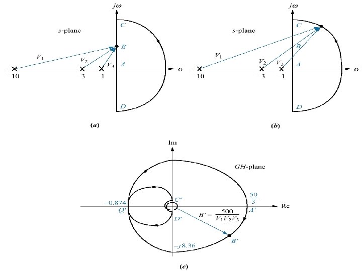
Vector evaluation of the Nyquist diagram for Example 10. 4 a. vectors on contour at low frequency; b. vectors on contour around infinity; c. Nyquist diagram The Nyquist Diagram is plotted by substituting the points of the contour shown in Figure (a) into G(s) = 500/[(s+1)(s+3)(s+10)] It’s performing complex arithmetic using vectors of G(s) drawn to points of the contour as shown in (a) and (b) The resultant vector, R, found at any point is the product of zero vectors divided by product of pole vectors as in (c)

Vector evaluation of the Nyquist diagram for Example 10. 4 a. vectors on contour at low frequency; b. vectors on contour around infinity; c. Nyquist diagram Evaluating G(s) at specified points we get So from A to C the magnitude is finite goes from 50/3 to 0 and the angle goes from 0 to -270 o From C to D the magnitude is 0 while there is an angle change of 540 o so goes from -270 o to 270 o

Vector evaluation of the Nyquist diagram for Example 10. 4 The mapping can be explained analytically by Substituting s= jω and evaluating G(jω) at specified points Multiplying numerator and denominator by the complex conjugate of denominator, we obtain At 0 freq G(jω)=500/30= 50/3. Thus Nyquist diagram starts at 50/3 at an angle 0. As ω increases, the real part remains positive while imaginary part remains negative. At ω = √ 30/14, the real part becomes negative. At ω=√ 43 the Nyquist diagram crosses the negative real axis, the value at the crossing is -0. 874. Continuing toward ω = ∞, the real part is negative and imaginary is positive. At ω = ∞, G(jω)≈500 j/ω3 or approximately 0 at 90 o

Detouring around open-loop poles: a. poles on contour; b. detour right; c. detour left

Nyquist Diagram for open-loop function with poles on contour Problem: Sketch the Nyquist diagram of unity feedback system where G(s)= (s+2)/ S 2 Solution: The system two poles at origin are on the contour and must be by-passed as in (a). Mapping DE is mirror of AB a. Contour for Example 10. 5; b. Nyquist diagram for Example 10. 5

Demonstrating Nyquist stability: a. system; b. contour; c. Nyquist diagram We could set K=1 and position the critical point at -1/K rather than -1. Thus the critical point appears to move closer to the origin as K increases. For this example P=2, and the critical point must be encircled by the Nyquist diagram to yield N=2 and a stable system. The system is marginally stable if the Nyquist diagram intersect the real axis at -1 ( frequency at this point is the frequency at which the root locus crosses the jw axis. )

Range of gain for stability via Nyquist criterion Problem: for the unity feedback system with G(s) = K/[s(s+3)(s+5)], find the range for stability, instability and the value of gain for marginal stability. Solution: first set K=1 and sketch Nyquist diagram for the system. Using the contour shown in (a), for all points on the imaginary axis, a. Contour for Example 10. 6; b. Nyquist diagram Next find the point where the diagram intersects the negative real axis by setting the imaginary part equal to zero. We find. and real part = -0. 0083. Finally From the contour, P=0; for stability N must equal zero. So the system is stable if the critical point lies outside the contour. K can be increased by 1/0. 0083 =120. 5 before the diagram encircles -1. Hence for stability K<120. 5. for marginal stability K=120. 5 At this gain the frequency is

Stability via Mapping Only the Positive jω-axis The system is stable at low values of gain, unstable at high values. This system is stable for the range of loop gain, K, that ensures that the open -loop magnitude is less than unity at that frequency where the phase angle is 180 o. a. Contour and root locus of system that is stable for small gain and unstable for large gain; b. Nyquist diagram

Stability via Mapping Only the Positive jω-axis The system is stable at high values of gain, unstable at low values. This system is stable for the range of loop gain, K, that ensures that the open -loop magnitude is greater than unity at that frequency where the phase angle is 180 o. a. Contour and root locus of system that is unstable for small gain and stable for large gain; b. Nyquist diagram

Stability Design via mapping positive jw-axis Example Problem: for the unity feedback system with G(s) = K/[(s 2+2 s+2)(s+2)], find the range for stability, instability and the value of gain for marginal stability. Solution: since P=0, we want no encirclements of -1 for stability. Hence. A gain less than unity at +/- 180 is required. first set K=1 and sketch the portion of Nyquist diagram along the positive imaginary axis as shown in (a). We find the intersection with the negative real axis as Setting the imaginary part = zero, we find This closed loop system is stable if the magnitude of the frequency response is less than unity at 180 o. Hence, the system is stable foe K<20, unstable for K>20, and marginally stable for K=20 (frequency at marginal stability is ) and substituting yields real part –(1/20) =

Nyquist diagram showing gain and phase margins Gain margin, GM, The gain margin is the change in open-loop gain, expressed in decibels (d. B), required at 180 o of phase shift to make the closed-loop system unstable. Phase margin, , The phase margin is the change in open-loop phase shift required at unity gain to make the closed-loop system unstable. GM = 20 log a.

Finding gain and phase margins Problem: find the gain and phase margins of system of previous example. If K = 6. Solution: to find the gain margin, first find the frequency where the Nyquist diagram crosses the negative real axis. The Nyquist diagram crosses the real axis at frequency of. The real part is calculated to be -0. 3. Thus, the gain can be increased by (1/0. 3) =3. 33 before the real part becomes -1. Hence the gain margin is GM = 20 log 3. 33 = 10. 45 d. B. To find the phase margin, find the frequency for which the magnitude is unity. We need to solve the equation to find frequency = 1. 253 rad/s. at this freq. the phase angle is 112. 3 o. The difference between this angle and -180 o is 67. 7 o, which is the phase margin.

Range of gain for stability via Bode plots Problem: use Bode plots to determine range of K within which the unity feed-back system with G(s) = K/[(s+2)(s+4)(s+5)] is stable. Solution: The closed loop system will be stable if the frequency response has a gain less than unity when the phase is +/-180 o We sketch the Bode plots as shown. The lowfrequency gain of G(s)H(s) is found by setting s=0. So the Bode magnitude plot starts at K/40. For convenience let K = 40 so that the log-magnitude plot starts at 0 d. B. At frequency 7 rad/s, when phase is 180 o, the magnitude is -20 d. B. So an increase in gain of +20 d. B is possible before system becomes unstable. Since the gain plot was scaled for a gain of 40, +20 d. B(a gain of 10) represents the required increase in gain above 40. Hence, the gain for instability is 40 X 10 = 400. 0<K<400 for stability. Compare to actual results 378 at freq. 6. 16 rad/s.

Evaluating Gain and Phase Margins

Gain and Phase Margins from Bode plots Problem: If K =200 in the system of previous example, find the gain and phase margins Solution: The Bode plot in Figure is scaled to a gain of 40. If K=200, the magnitude plot would be 20 log 5 = 13. 98 d. B higher. At phase = 180, on the magnitude plot the gain is -20. So the gain margin = -20 +13. 98 = 6. 02 d. B To find phase margin, we look on the magnitude plot for freq where the gain is 0 d. B (-13. 98 d. B normalized) occurs at 5. 5 rad/s freq. At this freq the angle is 165 so the phase margin is 165 -(-180) = 15 degrees

Relation between Closed-Loop Transient and Closed-Loop Frequency Responses Using the open loop transfer function And closed-loop transfer function We evaluate the magnitude of the closedloop freq response as A representative sketch of the log plot is shown in the Figure

Relation between Closed-Loop Transient and Closed-Loop Frequency Responses To relate the peak magnitude to the damping ratio we find At a frequency, of Since damping ratio is related to percent overshoot we can plot MP vs. percent overshoot

Response Speed and Closed-Loop Frequency Response We can relate the speed of the time response ( as measured in settling time, rising time, and peak time) and the bandwidth , of the Frequency response. The Bandwidth is defined as the frequency at which the magnitude response curve is 3 d. B down from its value at zero frequency. The Bandwidth for a two-pole system can be found by finding that freq for M=1/√ 2 (that is -3 d. B)

Response Speed and Closed-Loop Frequency Response We relate And to settling time and peak time by substituting We get, Figure 10. 41 Normalized bandwidth vs. damping ratio for: a. settling time; b. peak time; c. rise time

Relation between Closed-Loop and Open-Loop Frequency Responses These circles are called constant M circles and are the locus of the closed-loop magnitude frequency response for unity feed back systems. If the polar frequency response of an open-loop function, G(s), is plotted and superimposed on top of the constant M circles, the closedloop magnitude frequency response is determined by each intersection of this polar plot with the M circles. Figure 10. 42 Constant M circles

Relation between Closed-Loop and Open-Loop Frequency Responses These circles are called constant N circles If the polar frequency response of an open-loop function, G(s), is plotted and superimposed on top of the constant N circles, the closed-loop phase response is determined by each intersection of this polar plot with the N circles. Figure 10. 43 Constant N circles

Closed-Loop frequency response from Open-Loop frequency response Problem Find the closed-loop frequency response of the unity feedback system using G(s)=50/[s(s+3)(s+6)] Solution Evaluate the open-loop frequency function The Polar plot of the open-loop freq response ( Nyquist diagram) is shown superimposed over the M and N circles in the Figure Nyquist diagram for Example 10. 11 and constant M and N circles

Closed-Loop frequency response from Open-Loop frequency response The closed-loop magnitude frequency response can now be obtained by finding the intersection of each point of the Nyquist plot with the M circles. While the closed-loop phase response can be obtained by finding the intersection of each point of the Nyquist plot with the N circles. The result is shown in the Figure. Closed-loop frequency response for Example 10. 11

Nichols Charts displays the constant M and N circles in d. B, so that changes in gain are as simple to handle as in the Bode plots. The chart is a plot of the open-loop magnitude in d. B vs. open-loop phase angle in degrees.

Nichols Charts Nichols chart with frequency response for G(s) = K/[s(s + 1)(s + 2)] superimposed. Values for K = 1 and K = 3. 16 are shown.

Relation Between Closed-Loop Transient and Open-Loop Frequency Responses

Steady-State Error Characteristics from Frequency Response For type 0 system (the initial slope is 0) For un-normalized un-scaled Bode plot, the low frequency magnitude is 20 log KP For type 1 system (the initial slope is -20 d. B/decade) For un-normalized un-scaled Bode plot, the intersection of the initial 20 d. B/decade slope with the frequency axis is KV For type 2 system (the initial slope is -40 d. B/decade) For un-normalized un-scaled Bode plot, the intersection of the initial 40 d. B/decade slope with the frequency axis is √Ka

Steady-State Error Characteristics from Frequency Response Example: For Bode Log plots shown, find system type, and static error constants Solution: In (a) system is type 0, since the initial slope is 0. And 20 log KP =25, or KP = 17. 78 In (b) system is type 1, since the initial slope is -20 d. B/decade. And the value of Kv is the value of frequency that the initial slope intersects at the zero d. B crossing of the frequency axis. Hence Kv = 0. 55 In (c) system is type 2, since the initial slope is -40 d. B/decade. And the value of √Ka is the value of frequency that the initial slope intersects at the zero d. B crossing of the frequency axis. Hence Ka = 32 = 9