IOEMFG 543 Chapter 14 General purpose procedures for

IOE/MFG 543 Chapter 14: General purpose procedures for scheduling in practice Section 14. 4: Local search (Simulated annealing and tabu search) 1

Introduction Constructive vs. improvement type algorithms n Constructive type n – Construct the schedule by, e. g. , adding one job at the time n Improvement type – Start with some complete schedule – Try to obtain a better schedule by manipulating the current schedule 2

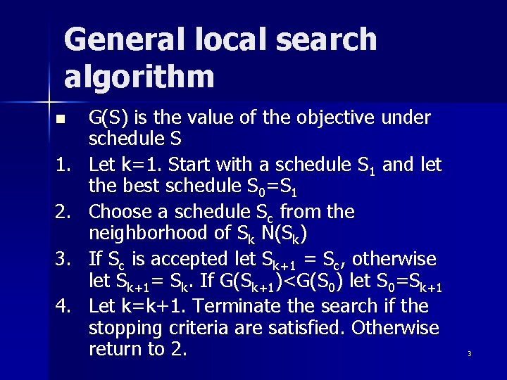
General local search algorithm n 1. 2. 3. 4. G(S) is the value of the objective under schedule S Let k=1. Start with a schedule S 1 and let the best schedule S 0=S 1 Choose a schedule Sc from the neighborhood of Sk N(Sk) If Sc is accepted let Sk+1 = Sc, otherwise let Sk+1= Sk. If G(Sk+1)<G(S 0) let S 0=Sk+1 Let k=k+1. Terminate the search if the stopping criteria are satisfied. Otherwise return to 2. 3

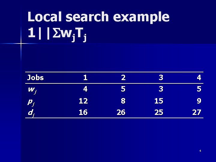
Local search example 1||Swj. Tj Jobs 1 2 3 4 wj 4 5 3 5 pj dj 12 8 15 9 16 26 25 27 4

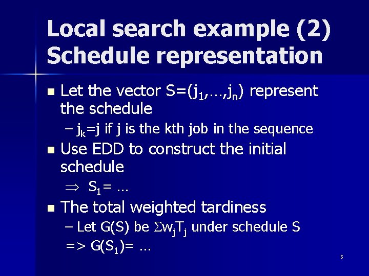
Local search example (2) Schedule representation n Let the vector S=(j 1, …, jn) represent the schedule – jk=j if j is the kth job in the sequence n Use EDD to construct the initial schedule Þ S 1= … n The total weighted tardiness – Let G(S) be Swj. Tj under schedule S => G(S 1)= … 5

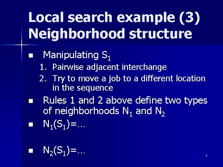
Local search example (3) Neighborhood structure n Manipulating S 1 1. Pairwise adjacent interchange 2. Try to move a job to a different location in the sequence n Rules 1 and 2 above define two types of neighborhoods N 1 and N 2 N 1(S 1)=… n N 2(S 1)=… n 6

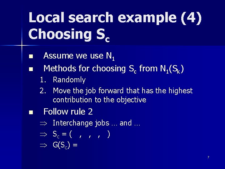
Local search example (4) Choosing Sc n n Assume we use N 1 Methods for choosing Sc from N 1(Sk) 1. Randomly 2. Move the job forward that has the highest contribution to the objective n Follow rule 2 Þ Þ Þ Interchange jobs … and … Sc = ( , , , ) G(Sc) = 7

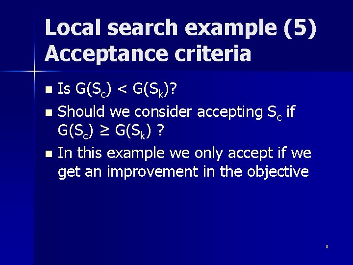
Local search example (5) Acceptance criteria Is G(Sc) < G(Sk)? n Should we consider accepting Sc if G(Sc) ≥ G(Sk) ? n In this example we only accept if we get an improvement in the objective n 8

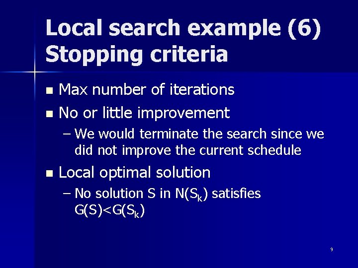
Local search example (6) Stopping criteria Max number of iterations n No or little improvement n – We would terminate the search since we did not improve the current schedule n Local optimal solution – No solution S in N(Sk) satisfies G(S)<G(Sk) 9

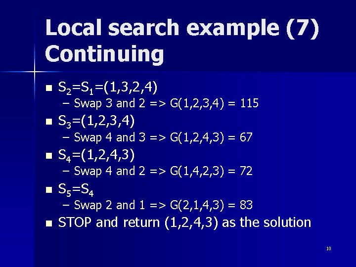
Local search example (7) Continuing n S 2=S 1=(1, 3, 2, 4) – Swap 3 and 2 => G(1, 2, 3, 4) = 115 n S 3=(1, 2, 3, 4) – Swap 4 and 3 => G(1, 2, 4, 3) = 67 n S 4=(1, 2, 4, 3) – Swap 4 and 2 => G(1, 4, 2, 3) = 72 n S 5=S 4 – Swap 2 and 1 => G(2, 1, 4, 3) = 83 n STOP and return (1, 2, 4, 3) as the solution 10

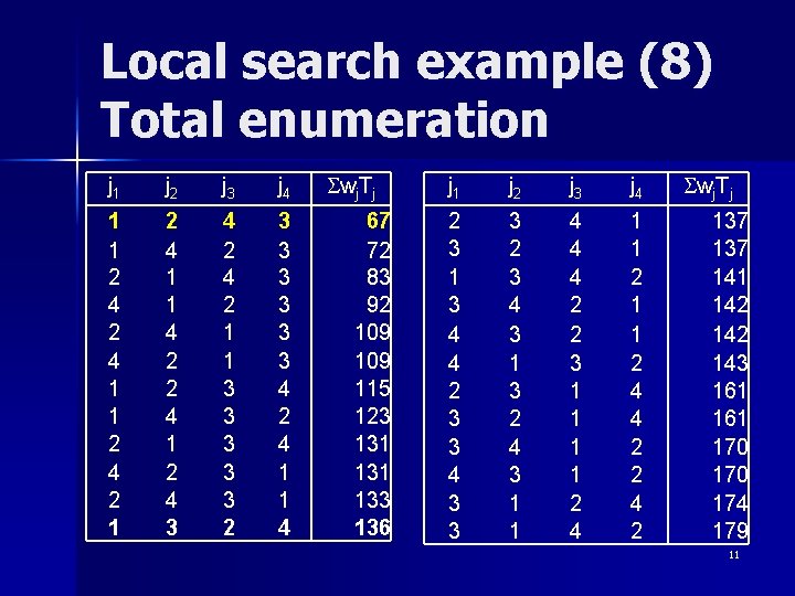
Local search example (8) Total enumeration j 1 j 2 j 3 j 4 1 1 2 4 2 1 2 4 1 1 4 2 2 4 1 2 4 3 4 2 1 1 3 3 3 2 3 3 3 4 2 4 1 1 4 Swj. Tj 67 72 83 92 109 115 123 131 133 136 j 1 j 2 j 3 j 4 2 3 1 3 4 4 2 3 3 4 3 3 3 2 3 4 3 1 3 2 4 3 1 1 4 4 4 2 2 3 1 1 2 4 4 2 2 4 2 Swj. Tj 137 141 142 143 161 170 174 179 11

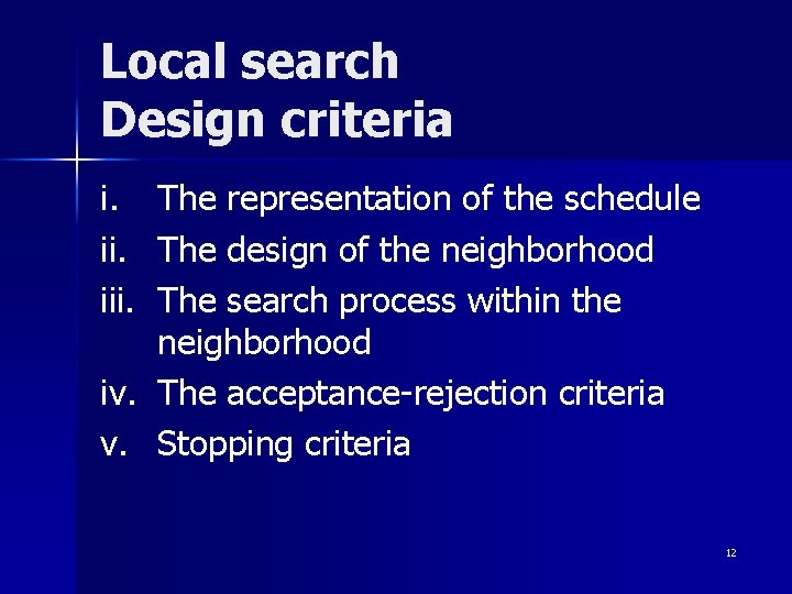
Local search Design criteria i. iii. The representation of the schedule The design of the neighborhood The search process within the neighborhood iv. The acceptance-rejection criteria v. Stopping criteria 12

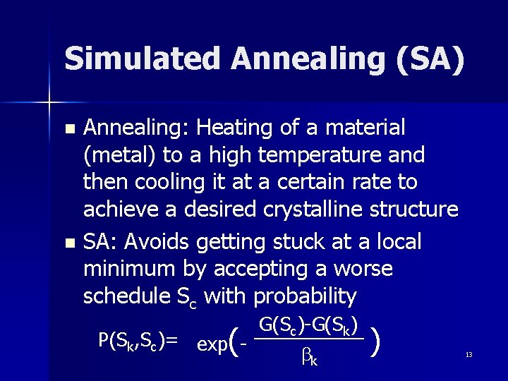
Simulated Annealing (SA) Annealing: Heating of a material (metal) to a high temperature and then cooling it at a certain rate to achieve a desired crystalline structure n SA: Avoids getting stuck at a local minimum by accepting a worse schedule Sc with probability n G(Sc)-G(Sk) P(Sk, Sc)= exp(bk ) 13

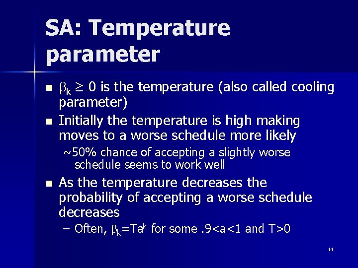
SA: Temperature parameter n n bk ≥ 0 is the temperature (also called cooling parameter) Initially the temperature is high making moves to a worse schedule more likely ~50% chance of accepting a slightly worse schedule seems to work well n As the temperature decreases the probability of accepting a worse schedule decreases – Often, bk=Tak for some. 9<a<1 and T>0 14

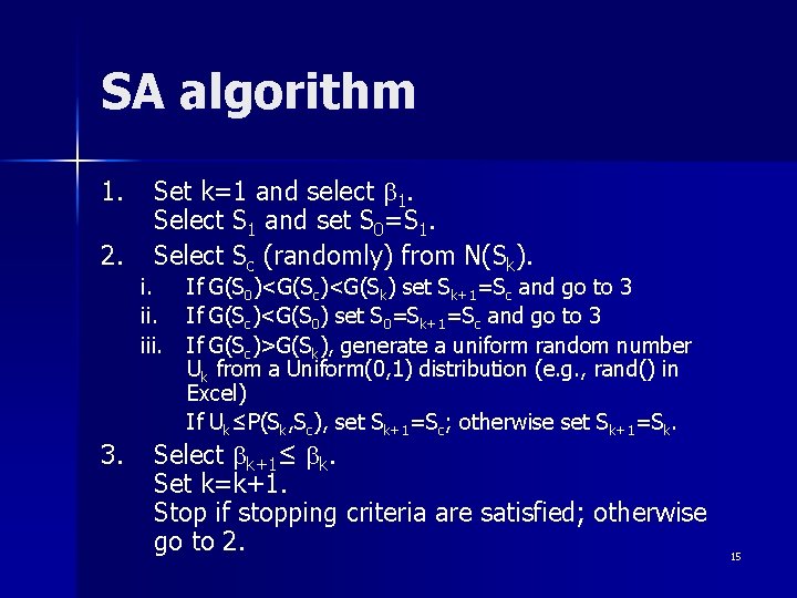
SA algorithm 1. 2. Set k=1 and select b 1. Select S 1 and set S 0=S 1. Select Sc (randomly) from N(Sk). i. iii. 3. If G(S 0)<G(Sc)<G(Sk) set Sk+1=Sc and go to 3 If G(Sc)<G(S 0) set S 0=Sk+1=Sc and go to 3 If G(Sc)>G(Sk), generate a uniform random number Uk from a Uniform(0, 1) distribution (e. g. , rand() in Excel) If Uk≤P(Sk, Sc), set Sk+1=Sc; otherwise set Sk+1=Sk. Select bk+1≤ bk. Set k=k+1. Stop if stopping criteria are satisfied; otherwise go to 2. 15

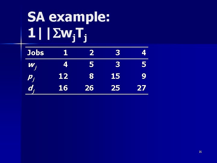
SA example: 1||Swj. Tj Jobs 1 2 3 4 wj 4 5 3 5 pj 12 8 15 9 dj 16 26 25 27 16

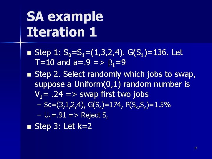
SA example Iteration 1 n n Step 1: S 0=S 1=(1, 3, 2, 4). G(S 1)=136. Let T=10 and a=. 9 => b 1=9 Step 2. Select randomly which jobs to swap, suppose a Uniform(0, 1) random number is V 1=. 24 => swap first two jobs – Sc=(3, 1, 2, 4), G(Sc)=174, P(Sk, Sc)=1. 5% – U 1=. 91 => Reject Sc n Step 3: Let k=2 17

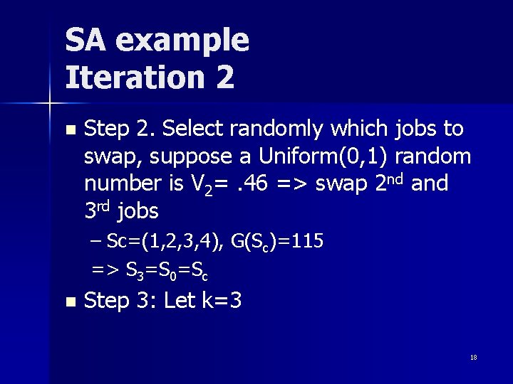
SA example Iteration 2 n Step 2. Select randomly which jobs to swap, suppose a Uniform(0, 1) random number is V 2=. 46 => swap 2 nd and 3 rd jobs – Sc=(1, 2, 3, 4), G(Sc)=115 => S 3=S 0=Sc n Step 3: Let k=3 18

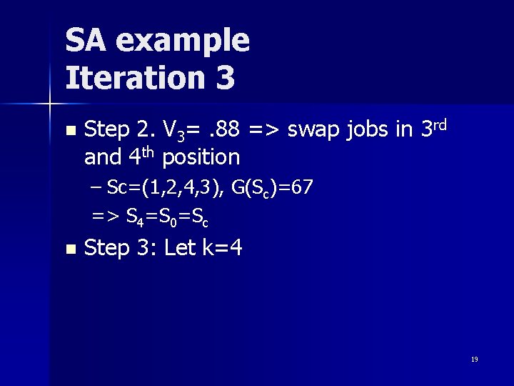
SA example Iteration 3 n Step 2. V 3=. 88 => swap jobs in 3 rd and 4 th position – Sc=(1, 2, 4, 3), G(Sc)=67 => S 4=S 0=Sc n Step 3: Let k=4 19

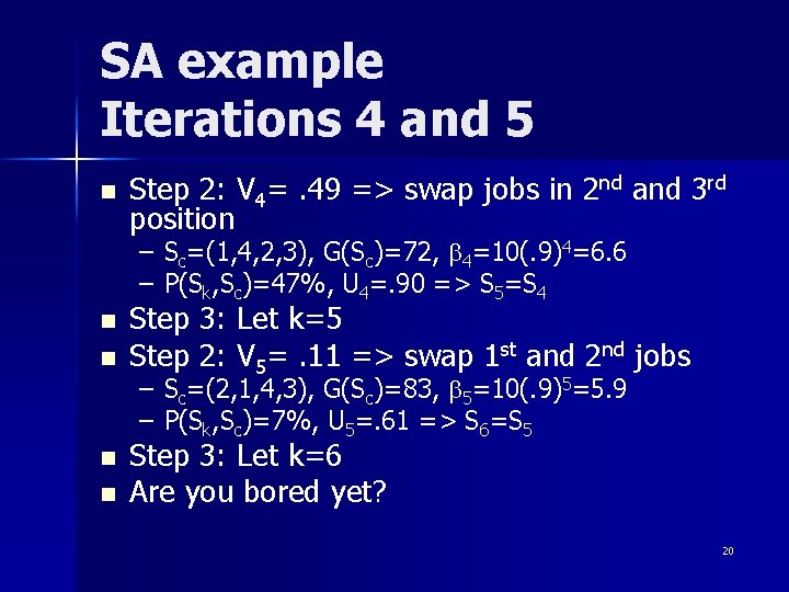
SA example Iterations 4 and 5 n Step 2: V 4=. 49 => swap jobs in 2 nd and 3 rd position – Sc=(1, 4, 2, 3), G(Sc)=72, b 4=10(. 9)4=6. 6 – P(Sk, Sc)=47%, U 4=. 90 => S 5=S 4 n n Step 3: Let k=5 Step 2: V 5=. 11 => swap 1 st and 2 nd jobs – Sc=(2, 1, 4, 3), G(Sc)=83, b 5=10(. 9)5=5. 9 – P(Sk, Sc)=7%, U 5=. 61 => S 6=S 5 Step 3: Let k=6 Are you bored yet? 20

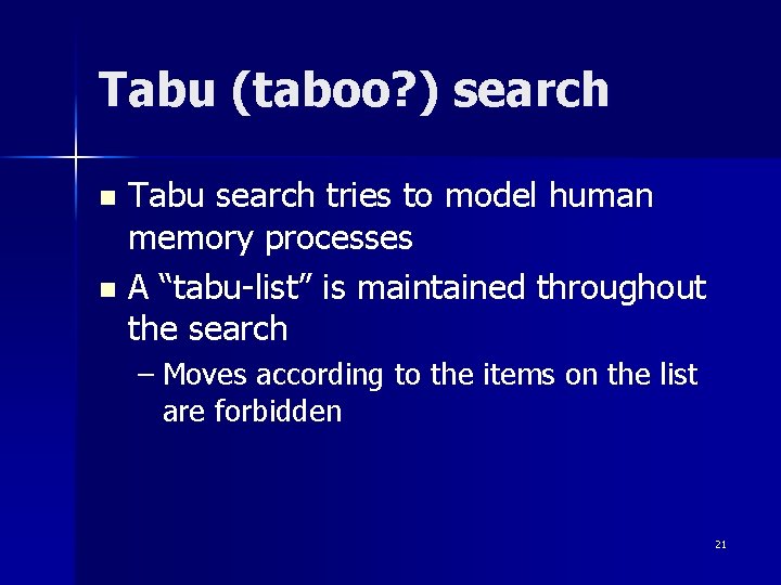
Tabu (taboo? ) search Tabu search tries to model human memory processes n A “tabu-list” is maintained throughout the search n – Moves according to the items on the list are forbidden 21

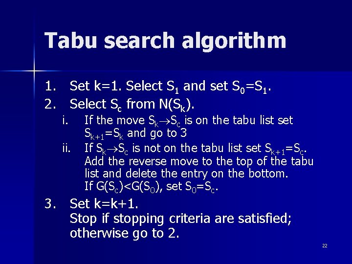
Tabu search algorithm 1. Set k=1. Select S 1 and set S 0=S 1. 2. Select Sc from N(Sk). i. ii. If the move Sk Sc is on the tabu list set Sk+1=Sk and go to 3 If Sk Sc is not on the tabu list set Sk+1=Sc. Add the reverse move to the top of the tabu list and delete the entry on the bottom. If G(Sc)<G(S 0), set S 0=Sc. 3. Set k=k+1. Stop if stopping criteria are satisfied; otherwise go to 2. 22

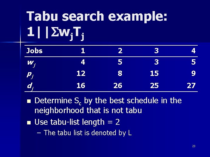
Tabu search example: 1||Swj. Tj Jobs 1 2 3 4 wj 4 5 3 5 pj 12 8 15 9 dj 16 26 25 27 n n Determine Sc by the best schedule in the neighborhood that is not tabu Use tabu-list length = 2 – The tabu list is denoted by L 23

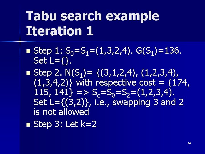
Tabu search example Iteration 1 Step 1: S 0=S 1=(1, 3, 2, 4). G(S 1)=136. Set L={}. n Step 2. N(S 1)= {(3, 1, 2, 4), (1, 2, 3, 4), (1, 3, 4, 2)} with respective cost = {174, 115, 141} => Sc=S 0=S 2=(1, 2, 3, 4). Set L={(3, 2)}, i. e. , swapping 3 and 2 is not allowed n Step 3: Let k=2 n 24

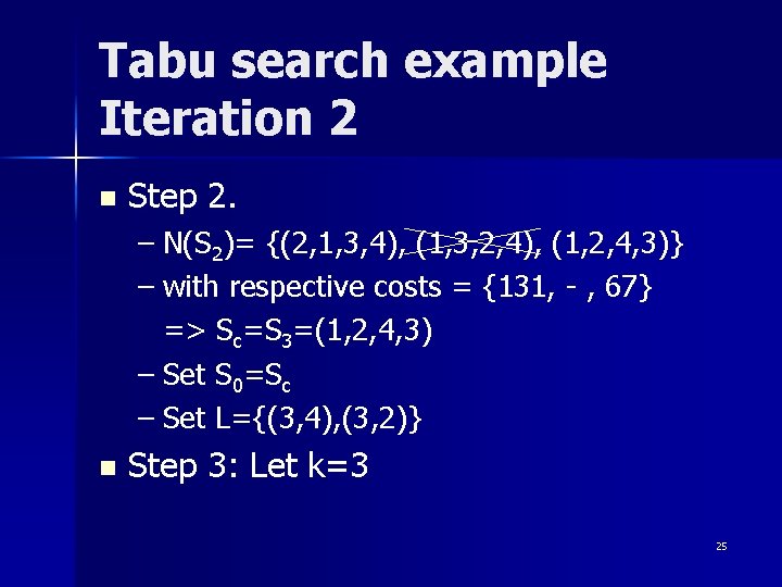
Tabu search example Iteration 2 n Step 2. – N(S 2)= {(2, 1, 3, 4), (1, 3, 2, 4), (1, 2, 4, 3)} – with respective costs = {131, - , 67} => Sc=S 3=(1, 2, 4, 3) – Set S 0=Sc – Set L={(3, 4), (3, 2)} n Step 3: Let k=3 25

Tabu search example Iteration 3 n Step 2 – N(S 3)= {(2, 1, 4, 3), (1, 4, 2, 3), (1, 2, 3, 4)} – with respective costs = {83, 72, -} => Sc=S 4=(1, 4, 2, 3) – Set L={(2, 4), (3, 4)} n Step 3: Let k=4 26

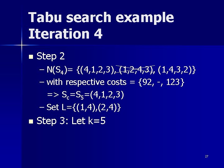
Tabu search example Iteration 4 n Step 2 – N(S 4)= {(4, 1, 2, 3), (1, 2, 4, 3), (1, 4, 3, 2)} – with respective costs = {92, -, 123} => Sc=S 5=(4, 1, 2, 3) – Set L={(1, 4), (2, 4)} n Step 3: Let k=5 27

Tabu search example Iteration 5 n Step 2 – N(S 5)= {(1, 4, 2, 3), (4, 2, 1, 3), (4, 1, 3, 2)} – with respective costs = {-, 109, 143} => Sc=S 6=(4, 2, 1, 3) – Set L={(2, 1), (4, 1)} n Step 3: Let k=6 28