IOEMFG 543 Chapter 3 Single machine models Sections

IOE/MFG 543 Chapter 3: Single machine models (Sections 3. 1 and 3. 2) 1

Sec. 3. 1: The total weighted completion time 1||S wj. Cj n Criteria for scheduling n Weighted shortest processing time first rule (WSPT) – order the jobs in decreasing order of wj /pj Theorem 3. 1. 1 – The WSPT is optimal for 1||S wj. Cj n – Shorter jobs processed first => more jobs finish early – The higher the weight the earlier a job should finish 2

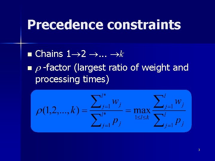
Precedence constraints Chains 1 2 . . . k n r -factor (largest ratio of weight and processing times) n 3

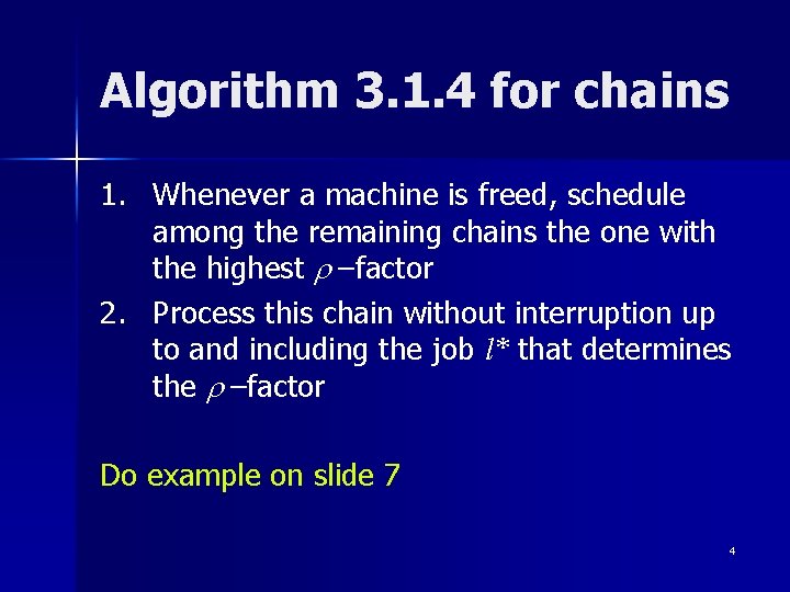
Algorithm 3. 1. 4 for chains 1. Whenever a machine is freed, schedule among the remaining chains the one with the highest r –factor 2. Process this chain without interruption up to and including the job l* that determines the r –factor Do example on slide 7 4

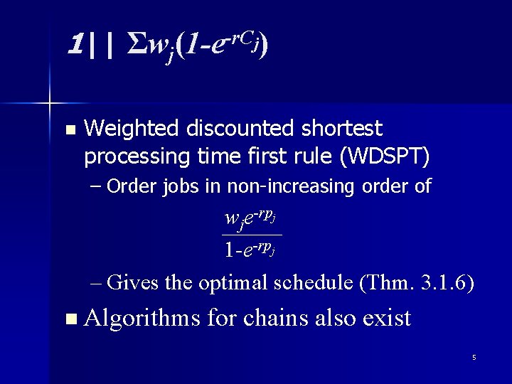
1|| Σwj(1 -e-r. Cj) n Weighted discounted shortest processing time first rule (WDSPT) – Order jobs in non-increasing order of wje-rpj 1 -e-rpj – Gives the optimal schedule (Thm. 3. 1. 6) n Algorithms for chains also exist 5

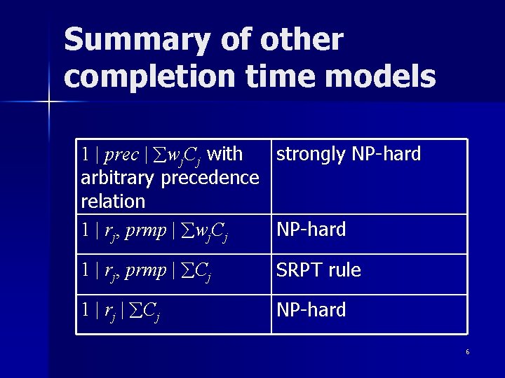
Summary of other completion time models 1 | prec | wj. Cj with strongly NP-hard arbitrary precedence relation 1 | rj, prmp | wj. Cj NP-hard 1 | rj, prmp | Cj SRPT rule 1 | rj | Cj NP-hard 6

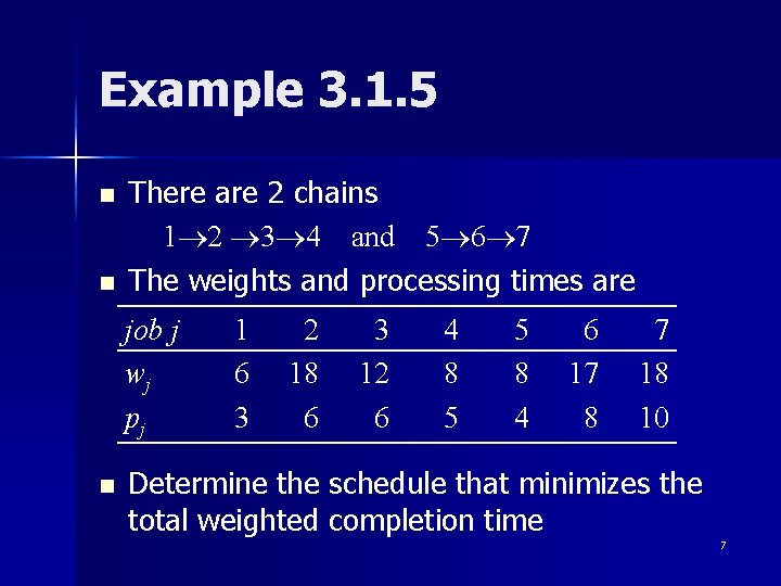
Example 3. 1. 5 n n There are 2 chains 1 2 3 4 and 5 6 7 The weights and processing times are job j wj pj n 1 6 3 2 18 6 3 12 6 4 8 5 5 8 4 6 17 8 7 18 10 Determine the schedule that minimizes the total weighted completion time 7

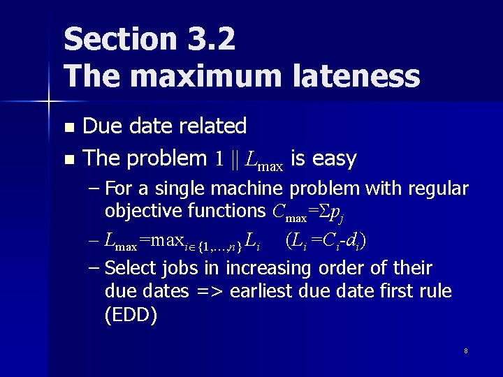
Section 3. 2 The maximum lateness Due date related n The problem 1 || Lmax is easy n – For a single machine problem with regular objective functions Cmax=Spj – Lmax=maxi {1, …, n} Li (Li =Ci-di) – Select jobs in increasing order of their due dates => earliest due date first rule (EDD) 8

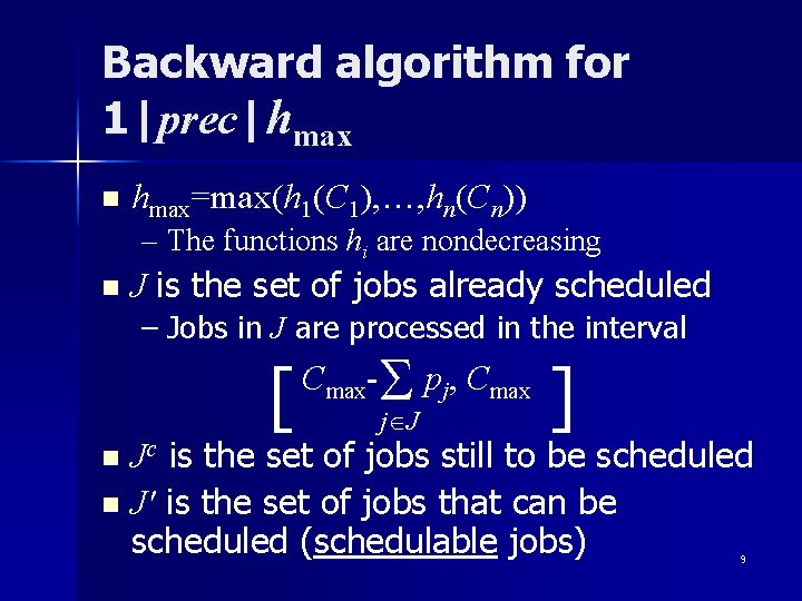
Backward algorithm for 1|prec|hmax n hmax=max(h 1(C 1), …, hn(Cn)) – The functions hi are nondecreasing n J is the set of jobs already scheduled – Jobs in J are processed in the interval [ S p, C ] j J Cmax- j max Jc is the set of jobs still to be scheduled n J' is the set of jobs that can be scheduled (schedulable jobs) n 9

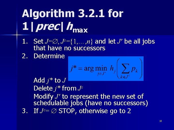
Algorithm 3. 2. 1 for 1|prec|hmax 1. Set J= , Jc={1, …, n} and let J' be all jobs that have no successors 2. Determine Add j* to J Delete j* from Jc Modify J' to represent the new set of schedulable jobs (have no successors) 3. If Jc= STOP, otherwise go to 2 10

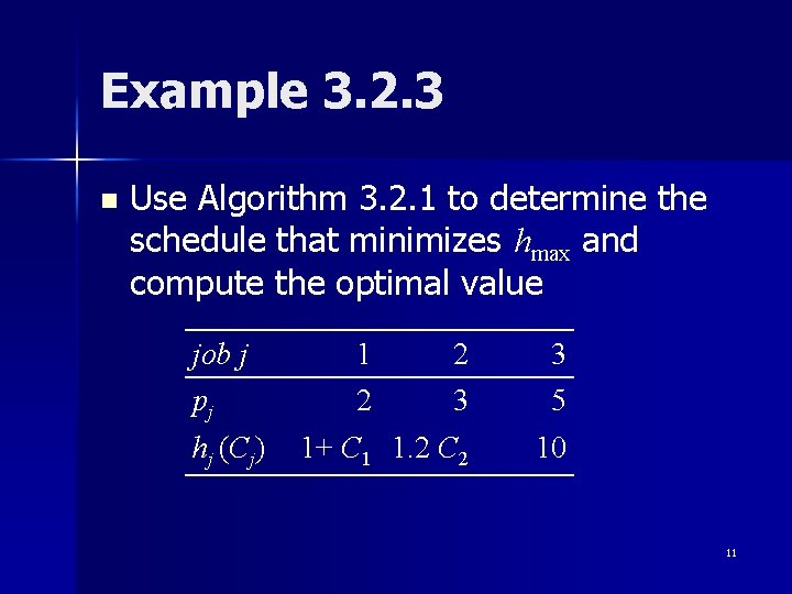
Example 3. 2. 3 n Use Algorithm 3. 2. 1 to determine the schedule that minimizes hmax and compute the optimal value job j pj hj (Cj) 1 2 2 3 3 5 1+ C 1 1. 2 C 2 10 11

Theorem 3. 2. 2. n n Algorithm 3. 2. 1. yields an optimal schedule for 1 | prec | hmax Proof: 12

Release dates 1 | rj | Lmax Significantly harder than 1 | prec | Lmax n It may be optimal to keep the machine idle to wait for the release of a new job (not a nondelay schedule) n Theorem 3. 2. 4. n – The problem 1 | rj | Lmax is strongly NP-hard – Reduces from 3 -PARTITION 13

Branch and bound n A method of effective enumeration – Generate a node tree n n n Compute the objective of a feasible schedule (feasible node) Compute lower bounds for a class of schedules (node) The node can be eliminated if the lower bound is higher than the cost of a schedule obtained earlier 14

Branch and bound for 1 | rj | Lmax n Branching – Level 0: single node and no jobs have been scheduled – Level 1: n nodes such that job j is scheduled first at node j – Level k: jobs in the first k positions have been specified 15

Branch and bound for 1 | rj | Lmax (2) n Branching – At a node let J be the set of jobs that have not been scheduled – Also let t be the time when a job can start processing at the node – Only create a node for job j at the node if rj<minl J(max(t, rl)+pl) 16

Branch and bound for 1 | rj | Lmax (3) n Bounding – At each node compute the optimal value using 1 | rj , prmp | Lmax for the remaining jobs – Preemptive EDD rule is optimal for 1 | rj , prmp | Lmax – If the preemptive solution gives a nonpreemptive schedule then it is feasible 17

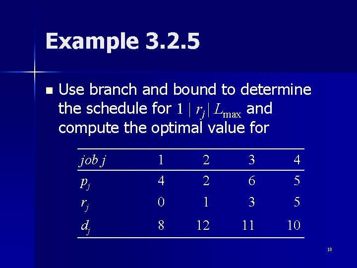
Example 3. 2. 5 n Use branch and bound to determine the schedule for 1 | rj | Lmax and compute the optimal value for job j pj 1 4 2 2 3 6 4 5 rj 0 1 3 5 dj 8 12 11 10 18