IOEMFG 543 Chapter 14 General purpose procedures for

IOE/MFG 543 Chapter 14: General purpose procedures for scheduling in practice Sections 14. 1 -14. 3: Dispatching rules and filtered beam search 1

Motivation n So far we have (mostly) discussed algorithms for obtaining an optimal solution for a specific problem Many scheduling problems are difficult to solve in practice Important to have general methods that can give good schedules in a relatively short amount of time 2

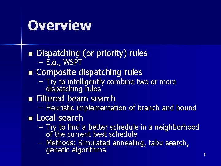
Overview n Dispatching (or priority) rules n Composite dispatching rules n Filtered beam search n Local search – E. g. , WSPT – Try to intelligently combine two or more dispatching rules – Heuristic implementation of branch and bound – Try to find a better schedule in a neighborhood of the current best schedule – Methods: Simulated annealing, tabu search, genetic algorithms 3

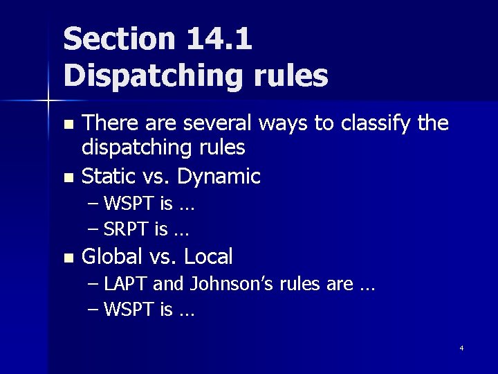
Section 14. 1 Dispatching rules There are several ways to classify the dispatching rules n Static vs. Dynamic n – WSPT is … – SRPT is … n Global vs. Local – LAPT and Johnson’s rules are … – WSPT is … 4

Applicability of elementary dispatching rules n Dispatching rules can work well when there is only a single objective – See Table 14. 1 page 337 for a list of rules and in what environments they tend to work well (sometimes optimal) n More sophisticated rules can often do better – Minimizing a combination of objectives – The objective can change with time and with the jobs waiting to be processed 5

Section 14. 2 Composite dispatching rules (CDR) n n n A CDR is a ranking expression that combines two or more elementary dispatching rules An elementary rule is a function of attributes of jobs and/or machines Each elementary rule has a scaling parameter – Depends on the attributes – E. g. , compute statistics for the set of jobs (are the due dates tight? ) 6

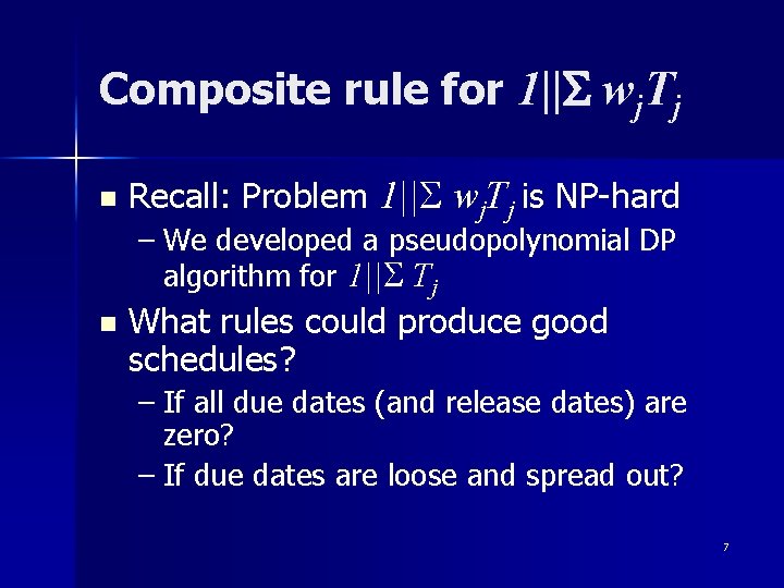
Composite rule for 1||S wj. Tj n Recall: Problem 1||S wj. Tj is NP-hard – We developed a pseudopolynomial DP algorithm for 1||S Tj n What rules could produce good schedules? – If all due dates (and release dates) are zero? – If due dates are loose and spread out? 7

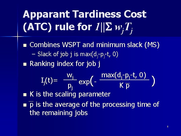
Apparant Tardiness Cost (ATC) rule for 1||S wj. Tj n Combines WSPT and minimum slack (MS) – Slack of job j is max(dj-pj-t, 0) n Ranking index for job j n wj max(dj-pj-t, 0) Ij(t)= exp() pj Kp K is the scaling parameter p is the average of the processing time of the remaining jobs n 8

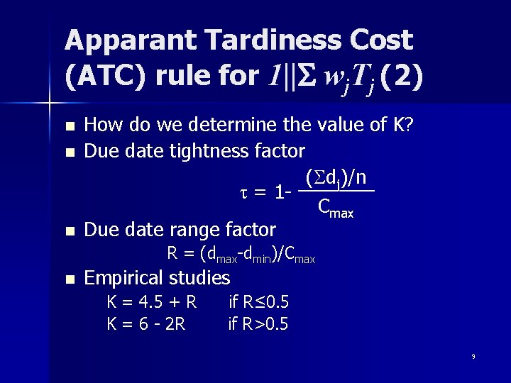
Apparant Tardiness Cost (ATC) rule for 1||S wj. Tj (2) n n n How do we determine the value of K? Due date tightness factor (Sdj)/n t = 1 Cmax Due date range factor R = (dmax-dmin)/Cmax n Empirical studies K = 4. 5 + R K = 6 - 2 R if R≤ 0. 5 if R>0. 5 9

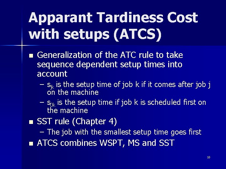
Apparant Tardiness Cost with setups (ATCS) n Generalization of the ATC rule to take sequence dependent setup times into account – sjk is the setup time of job k if it comes after job j on the machine – s 0 k is the setup time if job k is scheduled first on the machine n SST rule (Chapter 4) – The job with the smallest setup time goes first n ATCS combines WSPT, MS and SST 10

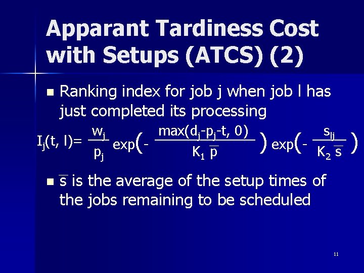
Apparant Tardiness Cost with Setups (ATCS) (2) n Ranking index for job j when job l has just completed its processing wj max(dj-pj-t, 0) Ij(t, l)= exp(pj K 1 p n slj ) exp(- K 2 s s is the average of the setup times of the jobs remaining to be scheduled 11 )

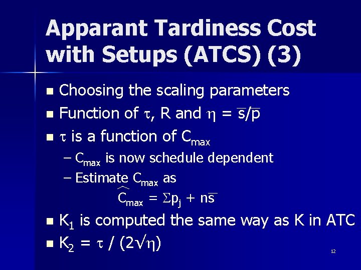
Apparant Tardiness Cost with Setups (ATCS) (3) Choosing the scaling parameters n Function of t, R and h = s/p n t is a function of Cmax n – Cmax is now schedule dependent – Estimate Cmax as Cmax = Spj + ns K 1 is computed the same way as K in ATC n K 2 = t / (2√h) n 12

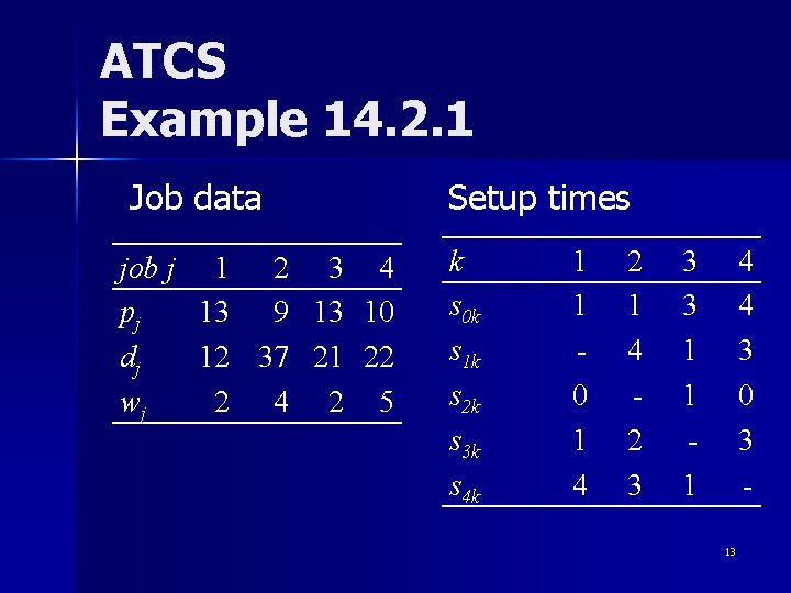
ATCS Example 14. 2. 1 Job data job j 1 2 3 4 pj 13 9 13 10 dj 12 37 21 22 wj 2 4 2 5 Setup times k s 0 k s 1 k s 2 k s 3 k s 4 k 1 1 0 1 4 2 3 3 3 1 1 1 4 4 3 0 3 13

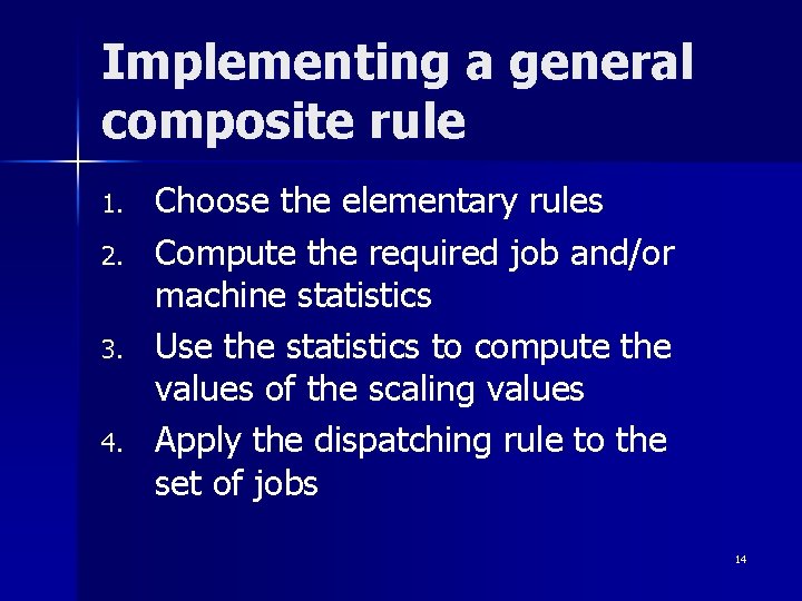
Implementing a general composite rule 1. 2. 3. 4. Choose the elementary rules Compute the required job and/or machine statistics Use the statistics to compute the values of the scaling values Apply the dispatching rule to the set of jobs 14

Section 14. 3 Filtered beam search (FBS) n Enumerative branch and bound is one of the most widely used procedures for solving NP-hard problems – It can be used to optimally solve any of the scheduling problems that we have considered so far n Problem: 15

Branch and bound (B&B) n n In branch and bound we can eliminate all nodes such that the lower bound is higher than the cost of the best feasible solution found so far Consequences: – If we can start off with a good solution then many nodes can potentially be eliminated n Bad news: – The number of nodes can still be large 16

Beam width FBS is a B&B-based method in which only some nodes at any given level are evaluated n Nodes that are not evaluated are discarded permanently n The number of nodes that are retained is called the beam width n 17

Filter width Evaluating each node at a given level can be computationally expensive n Instead, do a “crude prediction” of the quality of all nodes at a given level n Evaluate a number of nodes thoroughly n – This number is called the filter width 18

Crude prediction and thorough evaluation n Example of a crude prediction – Combine 1. 2. n The contribution to the objective of the jobs already scheduled Some job statistic, e. g. , due date factor Example of a thorough evaluation – Schedule the remaining jobs according to a composite dispatching rule – This gives an upper bound on the value at this node 19

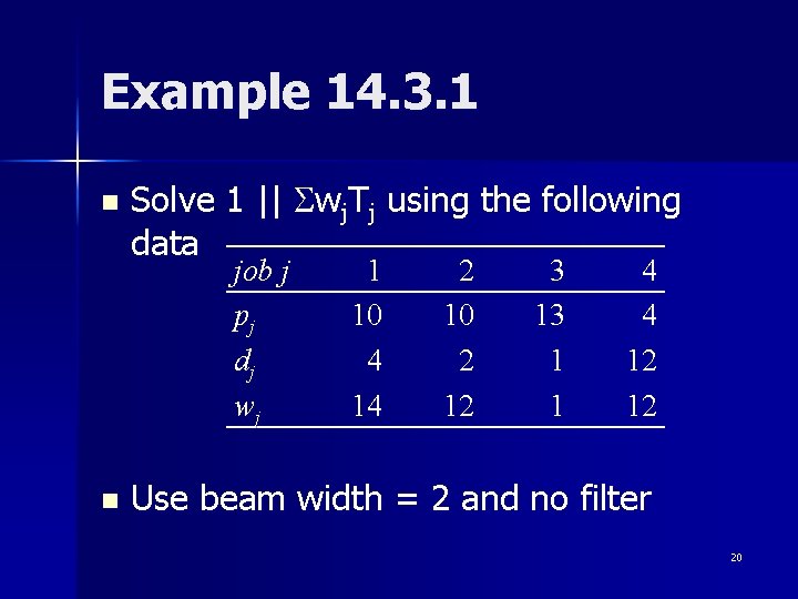
Example 14. 3. 1 n Solve 1 || Swj. Tj using the following data job j pj dj wj n 1 10 4 14 2 10 2 12 3 13 1 1 4 4 12 12 Use beam width = 2 and no filter 20