Introduction to Statistical Methods for Measuring Omics and

Introduction to Statistical Methods for Measuring “Omics” and Field Data PCA, Pco. A, distance measure, AMOVA

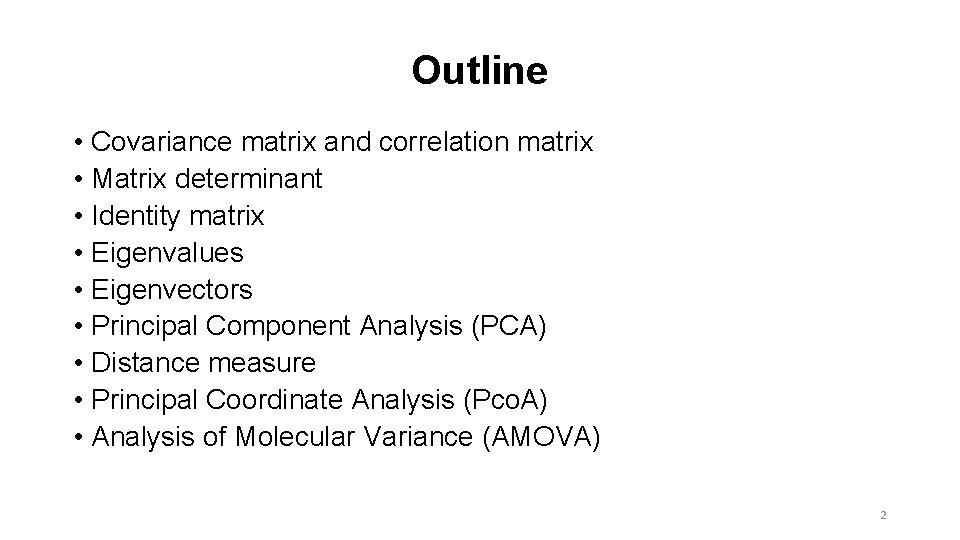
Outline • Covariance matrix and correlation matrix • Matrix determinant • Identity matrix • Eigenvalues • Eigenvectors • Principal Component Analysis (PCA) • Distance measure • Principal Coordinate Analysis (Pco. A) • Analysis of Molecular Variance (AMOVA) 2

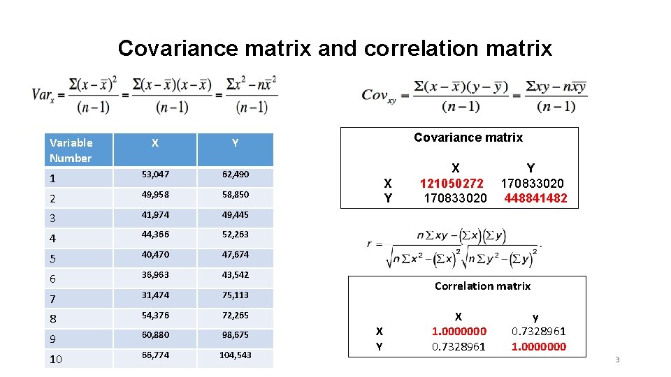
Covariance matrix and correlation matrix Variable Number X Y 1 53, 047 62, 490 2 49, 958 58, 850 3 41, 974 49, 445 4 44, 366 52, 263 5 40, 470 47, 674 6 36, 963 43, 542 7 31, 474 75, 113 8 54, 376 72, 265 9 60, 880 98, 675 10 66, 774 104, 543 Covariance matrix X Y X 121050272 170833020 Y 170833020 448841482 Correlation matrix X Y X y 1. 0000000 0. 7328961 1. 0000000 3

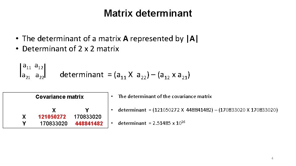
Matrix determinant • The determinant of a matrix A represented by |A| • Determinant of 2 x 2 matrix a 11 a 12 a 21 a 22 determinant = (a 11 X a 22) – (a 12 x a 21) Covariance matrix X Y X 121050272 170833020 Y 170833020 448841482 • The determinant of the covariance matrix • determinant = (121050272 X 448841482) – (170833020 X 170833020) • determinant = 2. 51485 x 1016 4

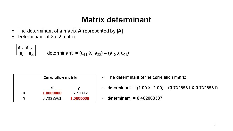
Matrix determinant • The determinant of a matrix A represented by |A| • Determinant of 2 x 2 matrix a 11 a 12 a 21 a 22 X Y determinant = (a 11 X a 22) – (a 12 x a 21) Correlation matrix • The determinant of the correlation matrix X y 1. 0000000 0. 7328961 1. 0000000 • determinant = (1. 00 X 1. 00) – (0. 7328961 X 0. 7328961) • determinant = 0. 462863307 5

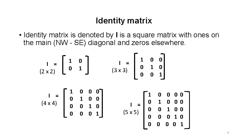
Identity matrix • Identity matrix is denoted by I is a square matrix with ones on the main (NW - SE) diagonal and zeros elsewhere. I = (2 x 2) I = (4 x 4) 1 0 0 1 0 0 I = (3 x 3) 0 0 1 0 0 1 1 0 I = 0 1 (5 x 5) 0 0 0 0 1 0 0 0 0 0 1 6

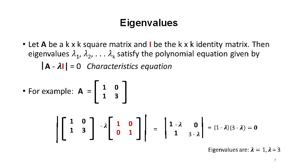
Eigenvalues • 1 1 0 3 1 0 0 1 = 1 0 1 = 7

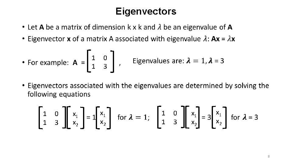
Eigenvectors • 1 0 1 3 x 1 x 2 8

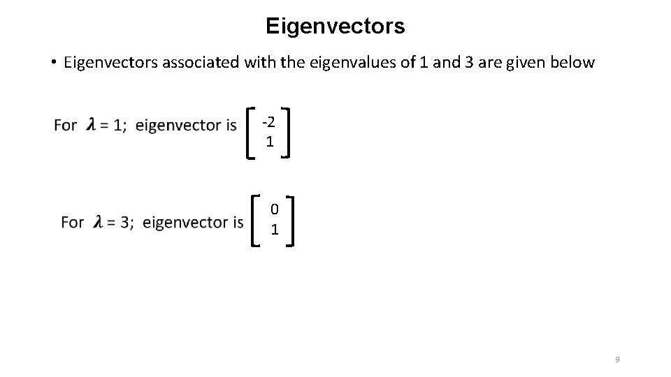
Eigenvectors • Eigenvectors associated with the eigenvalues of 1 and 3 are given below -2 1 0 1 9

Principal Component Analysis 10

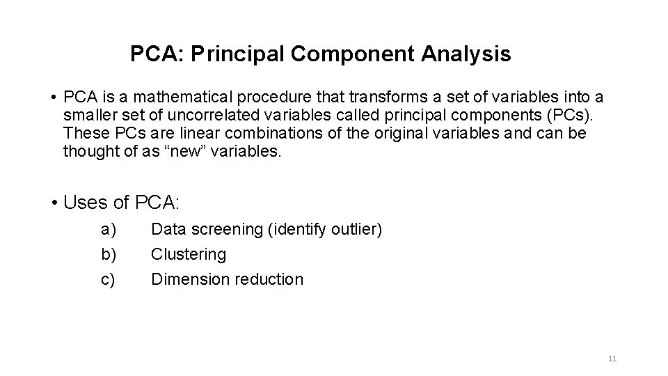
PCA: Principal Component Analysis • PCA is a mathematical procedure that transforms a set of variables into a smaller set of uncorrelated variables called principal components (PCs). These PCs are linear combinations of the original variables and can be thought of as “new” variables. • Uses of PCA: a) b) c) Data screening (identify outlier) Clustering Dimension reduction 11

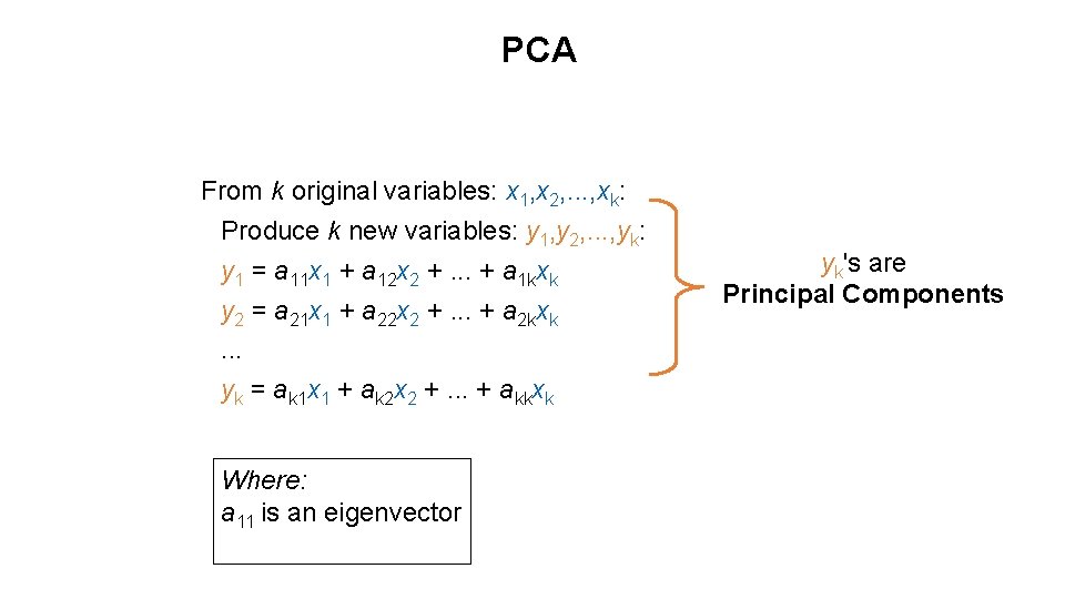
PCA From k original variables: x 1, x 2, . . . , xk: Produce k new variables: y 1, y 2, . . . , yk: y 1 = a 11 x 1 + a 12 x 2 +. . . + a 1 kxk y 2 = a 21 x 1 + a 22 x 2 +. . . + a 2 kxk. . . yk = ak 1 x 1 + ak 2 x 2 +. . . + akkxk Where: a 11 is an eigenvector yk's are Principal Components

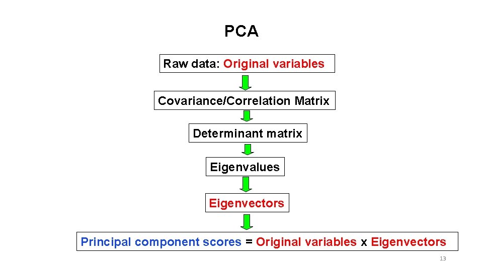
PCA Raw data: Original variables Covariance/Correlation Matrix Determinant matrix Eigenvalues Eigenvectors Principal component scores = Original variables x Eigenvectors 13

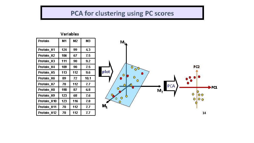
PCA for clustering using PC scores Variables Protein M 1 M 2 M 3 Protein_X 1 124 99 4. 3 Protein_X 2 106 67 7. 5 Protein_X 3 111 90 9. 2 Protein_X 4 109 90 7. 5 Protein_X 5 113 112 9. 6 Protein_X 6 89 72 10. 1 Protein_X 7 78 112 7. 7 Protein_X 8 190 87 6. 8 Protein_X 9 123 68 7. 6 Protein_X 10 123 116 7. 8 Protein_X 11 78 112 7. 7 Protein_X 12 78 112 7. 7 M 3 PC 2 plot M 2 PCA PC 1 M 1 14

Distance measures 15

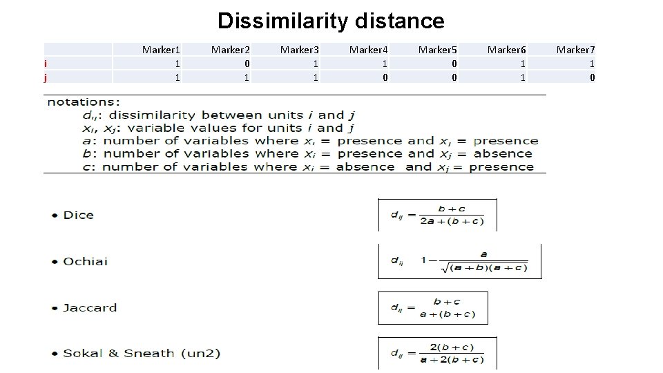
Similarity and Dissimilarity distance • Similarity distance measure: • Euclidean distance • Manhattan distance • Dissimilarity distance measure: • Jaccard • Dice 16

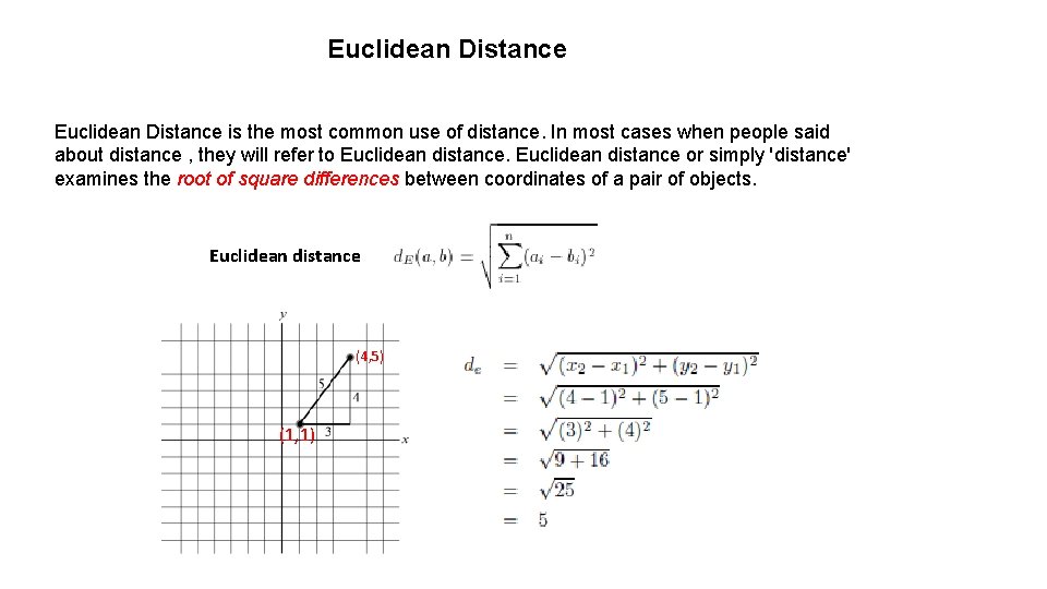
Euclidean Distance is the most common use of distance. In most cases when people said about distance , they will refer to Euclidean distance or simply 'distance' examines the root of square differences between coordinates of a pair of objects. Euclidean distance (4, 5) (1, 1)

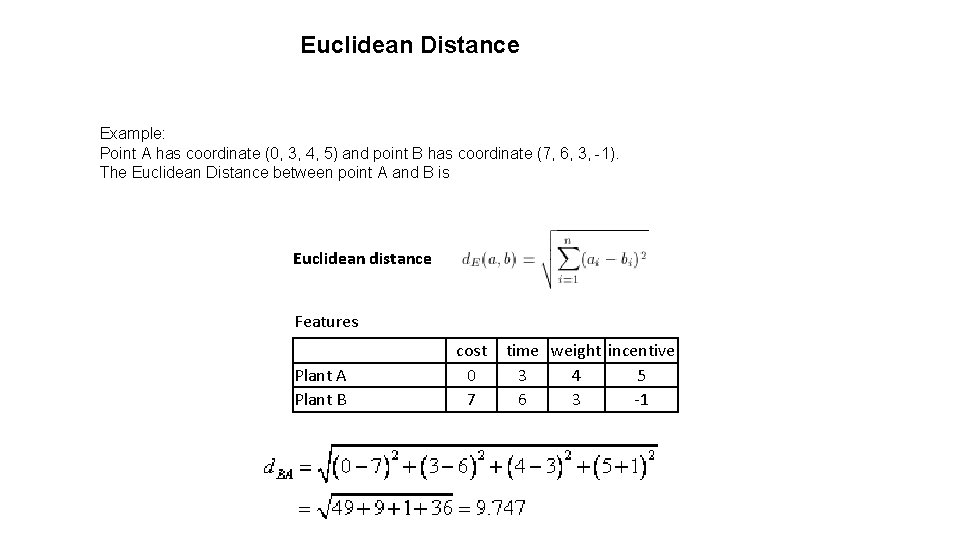
Euclidean Distance Example: Point A has coordinate (0, 3, 4, 5) and point B has coordinate (7, 6, 3, -1). The Euclidean Distance between point A and B is Euclidean distance Features Plant A Plant B cost time weight incentive 0 3 4 5 7 6 3 -1

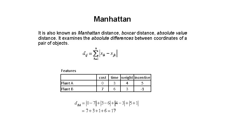
Manhattan It is also known as Manhattan distance, boxcar distance, absolute value distance. It examines the absolute differences between coordinates of a pair of objects. Features Plant A Plant B cost time weight incentive 0 3 4 5 7 6 3 -1

Dissimilarity distance i j Marker 1 1 1 Marker 2 0 1 Marker 3 1 1 Marker 4 1 0 Marker 5 0 0 Marker 6 1 1 Marker 7 1 0

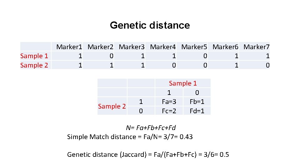
Genetic distance Sample 1 Sample 2 Marker 1 Marker 2 Marker 3 Marker 4 Marker 5 Marker 6 Marker 7 1 0 1 1 1 0 0 1 0 Sample 2 1 0 Sample 1 1 0 Fa=3 Fb=1 Fc=2 Fd=1 N= Fa+Fb+Fc+Fd Simple Match distance = Fa/N= 3/7= 0. 43 Genetic distance (Jaccard) = Fa/(Fa+Fb+Fc) = 3/6= 0. 5

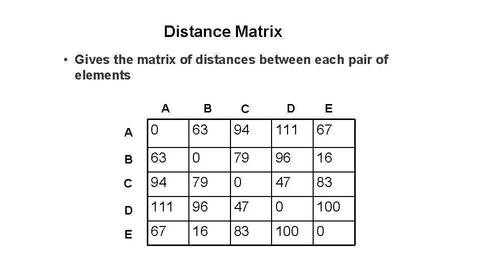
Distance Matrix • Gives the matrix of distances between each pair of elements A B C D E A 0 63 94 111 67 B 63 0 79 96 16 C 94 79 0 47 83 D 111 96 47 0 100 E 67 16 83 100 0

Principal Coordinate Analysis 23

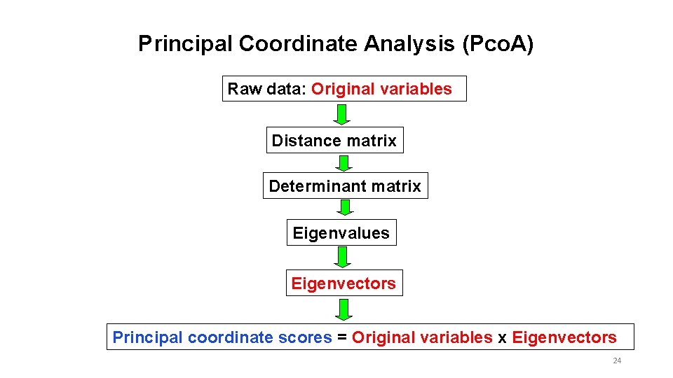
Principal Coordinate Analysis (Pco. A) Raw data: Original variables Distance matrix Determinant matrix Eigenvalues Eigenvectors Principal coordinate scores = Original variables x Eigenvectors 24

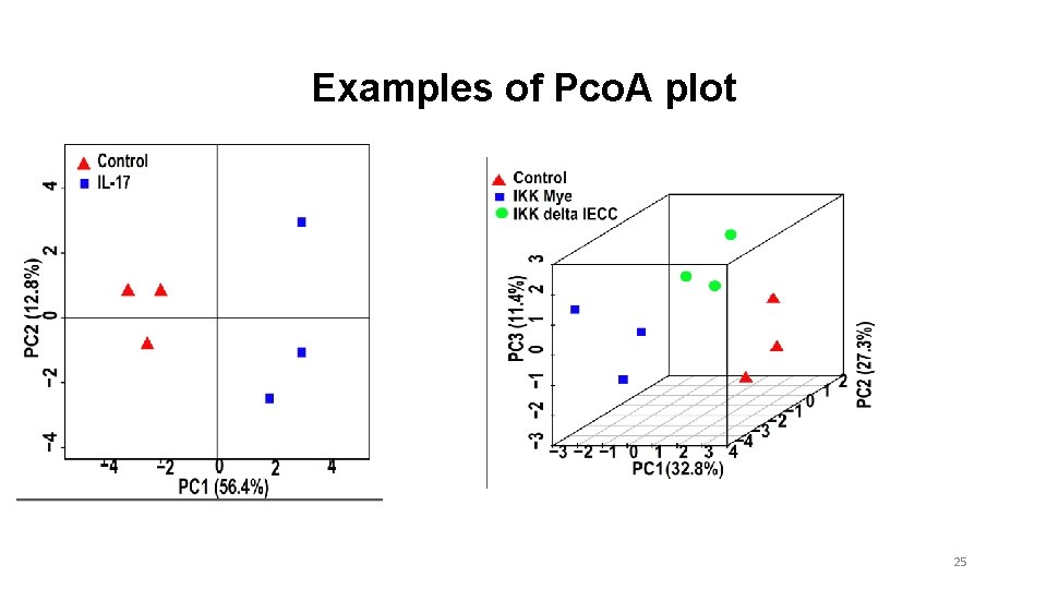
Examples of Pco. A plot 25

Analysis of molecular variance (AMOVA)

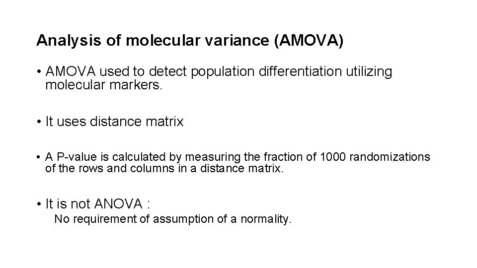
Analysis of molecular variance (AMOVA) • AMOVA used to detect population differentiation utilizing molecular markers. • It uses distance matrix • A P-value is calculated by measuring the fraction of 1000 randomizations of the rows and columns in a distance matrix. • It is not ANOVA : No requirement of assumption of a normality.

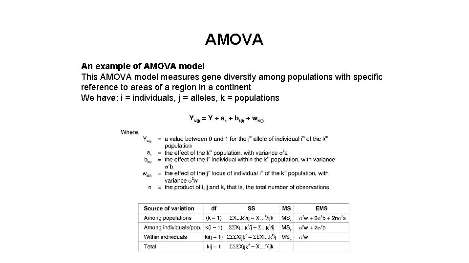
AMOVA An example of AMOVA model This AMOVA model measures gene diversity among populations with specific reference to areas of a region in a continent We have: i = individuals, j = alleles, k = populations

RStudio 29