Introduction to Static Program Analysis Mooly Sagiv Challenges

Introduction to Static Program Analysis Mooly Sagiv

Challenges in Proving Correctness • Specifying what the program is supposed to do • Writing loop invariants • Decision procedures for proving implications – Deduction

Static Analysis • Automatically infer sound invariants from the code • Prove the absence of certain program errors • Prove user-defined assertions • Report bugs before the program is executed

Simple Correct C code main() { int i = 0, *p =NULL, a[100]; for (i=0 ; i <100, i++) { a[i] = i; p = malloc(1, sizeof(int)); *p = i; free(p); // not alloc(p) p = NULL; // no leak }

Simple Correct C code main() { int i = 0, *p=NULL, a[100]; for (i=0 ; i <100, i++) { { 0 <= i < 100} a[i] = i; { p == NULL: } p = malloc(1, sizeof(int)); { alloc(p) } *p = i; {alloc(p)} free(p); {!alloc(p)} p = NULL; {p==NULL} }

Simple Incorrect C code main() { int i = 0, *p=NULL, a[100], j; for (i=0 ; i <j , i++) { { 0 <= i < j} a[i] = i; p = malloc(1, sizeof(int)); { alloc(p) } free(p); }

Sound (Incomplete) Static Analysis • It is undecidable to prove interesting program properties • Focus on sound program analysis – When the compiler reports that the program is correct it is indeed correct for every run – The compiler may report spurious (false alarms)

A Simple False Alarm int i, *p=NULL; … if (i >=5) { p = malloc(1, sizeof(int)); } … if (i >=5) { *p = 8; } … if (i >=5) { free(p); }

A Complicated False Alarm int i, *p=NULL; … if (foo(i)) { p = malloc(1, sizeof(int)); } … if (bar(i )) { *p = 8; } … if (zoo(i)) { free(p); }

Foundation of Static Analysis • Static analysis can be viewed as interpreting the program over an “abstract domain” • Execute the program over larger set of execution paths • Guarantee sound results – Whenever the analysis reports that an invariant holds it indeed hold

Even/Odd Abstract Interpretation • Determine if an integer variable is even or odd at a given program point

Example Program /* x=? */ while (x !=1) do { /* x=? */ if (x %2) == 0 /* x=? */ { x : = x / 2; } /* x=E */ else { x : = x * 3 + 1; /* x=O */ assert (x %2 ==0); } /* x=E */ } /* x=O*/

Lattice of Values ? O E

Abstract Interpretation Concrete Sets of stores Abstract Descriptors of sets of stores

Odd/Even Abstract Interpretation All concrete states {x: x Even} {0, 2} {0} ? {-2, 1, 5} {2} E O

Odd/Even Abstract Interpretation All concrete states {x: x Even}{-2, 1, 5} {0, 2} {0} {2} ? E O

Odd/Even Abstract Interpretation All concrete states {x: x Even}{-2, 1, 5} {0, 2} {0} {2} ? E O

Example Program while (x !=1) do { if (x %2) == 0 { x : = x / 2; } else /* x=E */ /* x=O */ { x : = x * 3 + 1; assert (x %2 ==0); } }

(Best) Abstract Transformer Operational Semantics Concrete Representation St Concretization Abstract Representation Concrete Representation Abstraction St Abstract Semantics Abstract Representation

(Best) Abstract Transformer x : = 3*x + 1 Concrete Representation St Concretization Abstract Representation Concrete Representation Abstraction x : = St 3*x + 1 x : = if x = then else if x = ? then ? else if x =O then E else O Abstract Representation

(Best) Abstract Transformer x : = 3*x + 1 - , …, -1, 0, 1, 2 …, St - , …, -2, 1, 7, …, Concretization Abstraction ? x : = St 3*x + 1 x : = if x = then else if x = ? then ? else if x =O then E else O ?

(Best) Abstract Transformer x : = 3*x + 1 - , …, -2 , 0, 2, 4 …, St - , …, -5, 1, 7, …, Concretization Abstraction E x : = St 3*x + 1 x : = if x = then else if x = ? then ? else if x =O then E else O O

(Best) Abstract Transformer x : = 3*x + 1 - , …, -1 , 1, 3 …, St - , …, -2, 4, 10, , Concretization Abstraction O x : = St 3*x + 1 x : = if x = then else if x = ? then ? else if x =O then E else O E

Runtime vs. Static Testing Effectiveness Runtime Static Analysis Missed Errors False alarms Locate rare errors Cost Proportional to program’s execution Proportional to program’s size No need to efficiently handle rare cases Can handle limited classes of programs and still be useful

Static Analysis Algorithms • Generate a control flow graph • Collecting semantics define the reachable states • Generate a system of equations over the abstract values at every node • Iteratively compute the simultaneous least solution at every node • The solution is guaranteed to be sound – Abstracts the set of reachable states – Computes an inductive invariant • May not be strong enough • The correctness of the safety properties can be conservatively checked

Example Interval Analysis • Find a lower and an upper bound of the value of a single variable • Can be generalized to multiple variables

Simple Correct C code main() { int i = 0, a[100]; { [-minint, maxint] } for (i=0 ; i <100, i++) { {[0, 99]} a[i] = i; {[0, 99]} } {[100, 100]}

The Power of Interval Analysis int f(x) { {[minint , maxint]} if (x > 100) { {[101, maxint]} return x -10 ; {[91, maxint-10]; } } else { {[minint, 100] } return f(f(x+11)) { [91, 91]} }

Example Program Interval Analysis n 1 x : = 1 ; while x 1000 do x : = x + 1; x : =1 n 2 x : =x+1 assume x>1000 assume x 1000 n 3 n 4

Example Program Interval Analysis x : = 1 ; while x x : =1 1000 do [1, 1001] x : = x + 1; [- , ] n 1 n 2 x : =x+1 [1, 1000] assume x>1000 [1001, 1001] n 4 assume x 1000 n 3

Collecting Interpretation • Defines the set of reachable states as the least solution to a systems of equations • Uniquely defined • But not necessarily computable

Collecting Semantics (Example) - , …, -1, 0, 1, n 1 x : =1 1001 1, 2, …, 1001 assume x>1000 n 2 n 4 x : =x+1 1, 2, …, 1000 assume x 1000 n 3

Collecting Semantics (Example) n 1 CS[n 1] =Z assume x>1000 CS[n 2] = x : = 1 CS[n 1] n 2 n 4 x : = x+1 assume x 1000 CS[n 3] = assume x 1000 3] 2] x>1000 CS[n 4] = CS[n assume n 3 CS[n ] x : =1 x : =x+1 2 : 2 Z 2 Z CS[n 1] x : = 1 = w. {1} Z x : = x+1 = w. {z+1 | z w Z } assume x>100 = w. Z assume x 100 = w. CS[n 2] CS[n 3] CS[n 4] {x |1 x 1001} {x |1 x 1000} {x |1 x 1001} {1002} {x |x 1000} {x |x 1001} {1001]

The Lattice of Intervals -

Galois Connection

Abstract Interpretation of Joins then l 1 else u 1 l 2 u 2 �� min l 1, l 2 max u 1, u 2 [l 1, u 1] �[l 2, u 2] =[min(l 1, l 2), max (u 1, u 2)]

Abstract Interpretation of Meets assume l 1 assume u 1 l 2 u 2 � max l 1, l 2 min u 1, u 2 [l 1, u 1] �[l 2, u 2] =[max(l 1, l 2), min (u 1, u 2)]

Abstract Interpretation of Atomic Statements #[l, u] = [l, u] �skip� #[l, u] = [1, 1] � x : = 1� #[l, u] = [l, u] + [1, 1] = [l + 1, u + 1] x : = x + 1� #[l, u] = assume x k�

Interval Analysis n 1 DF[n 1] =[- , ] DF[n 2] = x : = assume x>1000 n 2 n 4 1 #DF[n 1] assume x 1000 # x : =x+1 xx 100 : = x+1 DF[n 3] = assume # DF[n 3] 2] x>100 DF[n 4] = assume # n 3 DF[n 2] #: Z Z DF[n 1] DF[n 2] DF[n 3] DF[n 4] x : = 1 #= w. [1, 1] [- , ] [1, 1001] [1, 1000] [1001, 1001] x : = x+1 #= [l, u]. [l+1, [- , ] [1, 1000] [1, 1001] {1002} # u+1] assume x>100 = w. x : =1 assume x 100 #= w. Z [x |x 1000] {x |x 1001} {1001]

Solving the Equations • For programs with loops the equations have many solutions • Every solution is sound • Compute a minimal solution

An Example with Multiple Solutions n 1 x: =1 n 2 skip DF(n 1) = [- , ] DF(n 2) = x: =1 # DF(n 1) skip # DF(n 3) = skip # DF(n 2) n 3 DF[n 1] DF[n 2] DF[n 3] Comments [- , ] Maximal [- , ] [1, 1] Minimal [- , ] [1, 2] Solution [- , ] [1, 1] [1, 2] Not a solution

Computing Minimal Solution • Initialize the interval at the entry according to program semantics • Initialize the rest of the intervals to empty • Iterate until no more changes

Iterations Interval Analysis n 1 x : =1 n 2 x : =x+1 assume x>1000 n 4 assume x 1000 N n 3 DF[n 1] [- , ] DF[n 2] � DF[n 3] � n 1 n 2 [1, 1] n 3 n 2 n 3 [1, 1] [1, 2] DF[n 4] �

Iterative Algorithm Chaotic(G(V, E): Graph, s: Node, L: Lattice, : L, f: E (L L) ){ for each v in V to n do DF[v] : = df[v] = WL = {s} while (WL ) do select and remove an element u WL for each v, such that. (u, v) E do temp = f(e)(DF[u]) new : = DF[v] temp if (new DF[V]) then DF[v] : = new; WL : = WL {v}

Iterations Interval Analysis n 1 x : =x+1 N DF[n 1] [- , ] DF[n 2 DF[n 3] DF[n ] 4] � � � WL {n 1, n 2, n 3, n 4} n 1 n 2 [1, 1] n 3 n 2 n 3 {n 2, n 3, n 4} [1, 1] [1, 2] {n 2, n 4} {n 3, n 4} [1, 2] {n 2, n 4} assume x>1000 n 2 n 4 assume x 1000 n 3

Fixed Points f( ) f 2( ) • A monotone function f: L L where (L, , , ) is a complete lattice Red(f) • Fix(f) = { l: l L, f(l) = l} • Red(f) = {l: l L, f(l) l} • Ext(f) = {l: l L, l f(l)} Fix(f) gfp(f) – l 1 l 2 f(l 1 ) f(l 2 ) • Tarski’s Theorem 1955: if f is monotone then: – lfp(f) = Fix(f) = Red(f) Fix(f) – gfp(f) = Fix(f) = Ext(f) Fix(f) lfp(f) f 2( ) f( )

f#( ) a: f( (a)) (f#(a)) f 2( ) f#2( ) f(x) x f#(y) y gfp(f#) gfp(f) f(x)=x f#(y)=y lfp(f) lfp(f#) f#(y) y f( ) f#2( ) f#( ) f(x) x f 2( ) f( )

Lfp(f) f# f f# Lfp(f#) f f# Finite Height Case f

Accelerating Convergence • The Iterative algorithm can diverge when the domains contains infinite increasing chains • Sometimes can take long time

Widening • Accelerate the convergence of the iterative procedure by jumping to a more conservative solution • Heuristic in nature • But simple to implement

Widening for Interval Analysis • [c, d] = [c, d] • [a, b] [c, d] = [ if a c then a else - , if b d then b else ]

Iterations Interval Analysis with widening DF[n 1] =[- , ] DF[n 2] = DF[n 2] x : = 1 #DF[n 1] x : = x+1 # DF[n 3] n 1 x : =1 n 2 # DF[n 3] = assume x 100 DF[n 2] x>100 # DF[n 4] = assume N DF[n 2]DF[n 3] DF[n 1] DF[n 2] [- , ] � � DF[n 4] � x : =x+1 assume x 1000 WL {n 1, n 2, n 3, n 4} n 1 n 2 [1, 1] n 3 n 2 n 3 {n 2, n 3, n 4} [1, 1] [1, ] {n 2, n 4} {n 3, n 4} [1, 1000] assume x>1000 n 4 { n 4} n 3

Widening yk = yk f (yk) lfp(f) � y 2 = y 1 f (y 1) x 2= f 2( ) y 1= f( ) x 1 = f( ) x 0 =

Narrowing • Improve the precision of widened solution • Heuristic in nature • But simple to implement

Narrowing for Interval Analysis • [a, b] = [a, b] • [a, b] [c, d] = [ if a = - then c else a, if b = then d else b ]

Iterations with narrowing after widening DF[n 1] =[- , ] DF[n 2] = DF[n 2] x : = 1 #DF[n 1] x : = x+1 # DF[n 3] = assume x 100 # DF[n 2] x>100 # DF[n 4] = assume N DF[n ] DF[n 1] DF[n 2] 2 DF[n 3] DF[n 4] [- , ] n 2 n 3 [1, ] [1, 1000] [1001, ] [2, 1001] WL {n 1, n 2, n 3, n 4} { n 4} [1001, 1001] x : =1 n 2 assume x>1000 n 4 x : =x+1 assume x 1000 {n 2, n 3, n 4} [1, 1] n 1 {n 3, n 4} n 3

Numeric Abstract Domain Examples y y x y x x signs intervals octagons x 0 polyhedra x [a, b] x y c ai xi c

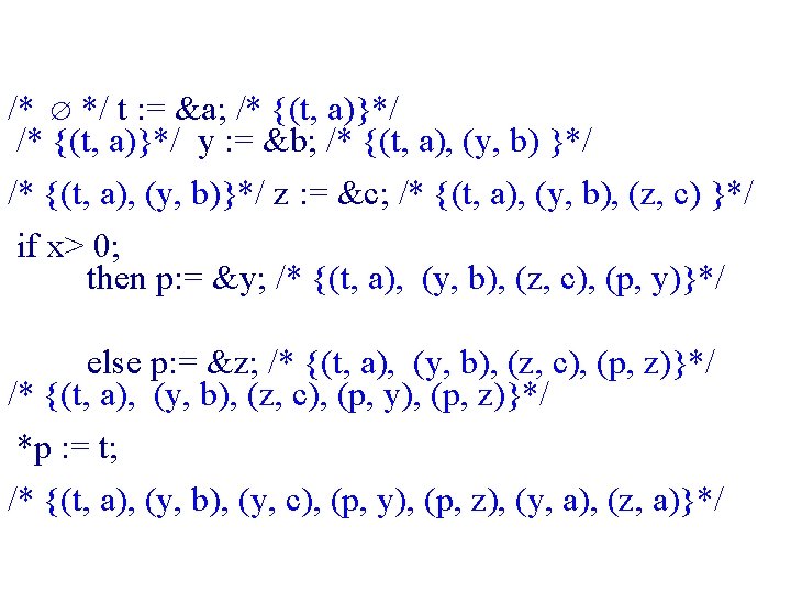
Pointer Language a : : = x | *x | &x | … b : : = true | a = a| not b assume b x : = a *x : = y

Collecting Semantics for Pointers State 1= [Loc Z]

Points-To Analysis u Lattice Lpt = u Galois connection u Meaning of statements

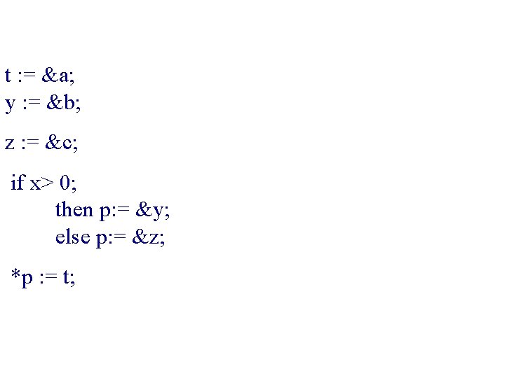
t : = &a; y : = &b; z : = &c; if x> 0 then p: = &y; else p: = &z; *p : = t;

Abstract Transformers State#= P(Var* Var*) x : = a # x : = &y # x : = *y # x : = y # *x : = y # assume x ==y # assume x !=y #

Flow insensitive points-to-analysis Steengard 1996 u Ignore control flow u One set of points-to per program u Can be represented as a directed graph u Conservative approximation – Accumulate pointers u Can be computed in almost linear time – Union find

Precision u We cannot usually have – (CS) = DF on all programs u But can we say something about precision in all programs?

The Join-Over-All-Paths (JOP) u Let paths(v) denote the potentially infinite set paths from start to v (written as sequences of edges) u For a sequence of edges [e 1, e 2, …, en] define f #[e 1, e 2, …, en]: L L by composing the effects of basic blocks f #[e 1, e 2, …, en](l) = f#(en) (… (f#(e 2) (f#(e 1) (l)) …) u JOP[v] = {f#[e 1, e 2, …, en]( ) [e 1, e 2, …, en] paths(v)}

JOP vs. Least Solution u The df solution obtained by Chaotic iteration satisfies for every v: – JOP[v] df[v] u A function f# is additive (distributive) if – f#( {x| x X}) = {f#(x) | X} u If every f# (u, v) is additive (distributive) for all the edges (u, v) – JOP[v] = df[v] u Examples – Intervals – Points-to

Notions of precision = (df) u (CS) = df u Meet(Join) over all paths u Using best transformers u Good enough u CS

Complexity of Chaotic Iterations u Usually depends on the height of the lattice u In some cases better bound exist u A function f is fast if f (f(l)) l f(l) u For fast functions the Chaotic iterations can be implemented in O(nest * |V|) iterations – nest is the number of nested loop – |V| is the number of control flow nodes

Success Stories Abstract Interpretation u SLAM: Microsoft Device Driver Verification u The Astrée Static Analyzer u Panaya Change Impact Analysis

Conclusion u Static analysis is powerful technique u But expensive – More efficient methods exist for structured programs u Abstract interpretation relates runtime semantics and static information u The concrete semantics serves as a tool in designing abstractions