Introduction to modelling in Health economics Melih Kaan

Introduction to modelling in Health economics Melih Kaan Sözmen MD, MSc.

What is a model? A simplification of reality to capture the ‘essence’ of the problem with the minimum level of complexity

Why use a model? To extend available information: to extrapolate results from short to long term to add cost data to outcome trials To generalise controlled trial circumstances to daily practice To synthesise data from multiple sources To extrapolate from intermediate to final outcomes To predict outcomes that are unknown or are unethical to collect Handle ambiguity of clinical data and variations in interpretation In case a quick (and relatively cheap) answer is necessary Is it cost effective to start a Rotavirus vaccination in Turkey?

Decision trees Markov Models

What is decision analysis Decision analysis is a quantitative, probabilistic way of modeling problems under situations of uncertainty

Elements of decision analysis 1. 2. 3. 4. 5. Identify and bound the problem Structure the problem Gather data Analyze the tree Perform sensitivity analysis

1. Identify the problem Decision model (usually decision tree) is chosen to represent the clinical problem Model needs to be simple enough to be understood, but complex enough to capture the essentials of the problem Many simplifying assumptions are needed for modeling

Example Suspected pulmonary embolism Given the patients history, signs and symptoms you are concerned that a pregnant woman may have PE. PE is life threatening event. Treatment with anticoagulation is effective in preventing further PE hence reducing fatality rate. However AC has a risk of major bleeding which can be fatal, it is better to avoid if unneccessary. Pulmonary angiography‐ can not be done because we have to avoid diagnostic methods using x‐ ray as she is pregnant Focus is survival of women

Step 1 Identify the problem What is the decision problem? What are the potential alternative actions? What events follow the decision? Should we treat with anticoagulant No anticoagulant Pulmonary embolism No pulmonary embolism‐ survive Dead

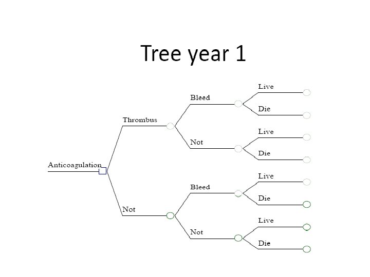
Step 2: Structure the problem Use a decision tree A tree depicts graphically the components decision of the decision problems and relates actions to consequences

Decision tree Nodes Decision node Chance node Terminal node

Decision node Represents available choices to decision maker Choices must be mutually exclusive To perform a test (or tests) To treat medically or surgically To do something now or later To do nothing at all In our example Treat with AC Do not treat with AC

Chance nodes are the temporal sequence of possible events which follow a decision node Chance events are out of the control of the decision maker ‐‐ they’re based on probability or outcome data Complication Each event at node is mutually exclusive They can not occur at the same time. . . The sum of event probabilities=1. 0 No complication

Terminal nodes Endpoints of decision problem The terminal health states Live Dead Values assigned to terminal states Live=1. 0 Dead=0 Can assign monetary values Live Complication Die

Example‐decision tree Probabilities Leaves Or terminal nod Decision node Branches Chance node

Example decision‐tree‐I Decision tree is averaged out to get the expected value (EV) for each strategy (from decision node) EV is the sum of products of the estimates of probability of events and their outcomes (payoff) EV = 0. 5 x 100 + 0. 5 x 0 = £ 50

Step 3 Gather Data Literature Can use RCTs, meta‐analysis Expert opinion

Step 3 Gather Data

AC or no AC? Fatal PE/hemorrhage (p=0. 01) PE(p=0. 19) AC Cost=500 Survive (p=0. 99) No PE(p=0. 81) Fatal hemorrhage (p=0. 008) Survive (p=0. 992) Fatal PE(p=0. 25) PE(p=0. 19) No AC Cost=100 Survive(p=0. 75) No PE(p=0. 81) 0 1 0 1 1

Step 4 Analysing the tree Calculate expected value of each strategy Also referred to as “rolling back” or taking the average of the tree Start at terminal node and multiply probabilities as you trace tree to origin to get probability of outcome Sum weighted outcomes for each strategy

AC or no AC? Eu=(0. 81*0. 992)+ (0. 990*0. 19)= 0. 9916 AC Cost=500 Eu=(0. 81*1. 0)+ (0. 75*0. 19)= 0. 94 0. 990 PE(p=0. 19) 0. 992 No PE(p=0. 81) 0. 750 Survive (p=0. 99) Fatal PE/hemorrhage (p=0. 008) Survive(p=0. 992) Fatal PE/hemorrhage (p=0. 25) PE(p=0. 19) No AC Cost=100 Fatal PE/hemorrhage (p=0. 01) Survive(p=0. 75) No PE(p=0. 81) 0 1 0 1 1

Sensitivity analysis Perform 1‐way sensitivity analyses on all parameters to debug tree Vary probabilities from 0 to 1 response of model to changes should be logical

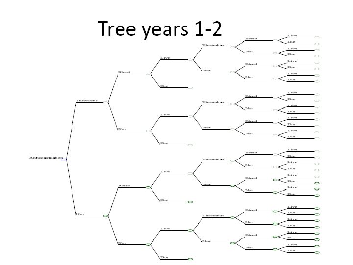
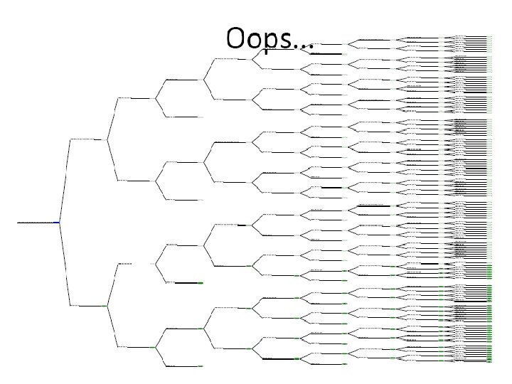
When to use Markov Model Transitions into and out of health states are possible, e. g. , recurrent events MI, stroke, Cancer Modeling a complex disease Probabilities vary over time The timeframe of the analysis is lengthy A decision tree would become too complex

Markov modelling Probability of going to a state depends only on current state, not on history The states that can be distinghuised are different regarding costs and value of health

Markov structure HEALTHY ILL DEAD CYCLETIME HEALTHY ILL DEAD

Markov model 49 2 14 12 6 7

Example Markov Model Cycles patients through health states based on state specific probabilities Example model: Healthy Sick Dead Each state is assigned its own utility and cost

Summary of Therapies Therapy Standard of care New treatment Cost of treatment, one month $800 $1, 500 Progression from healthy to sick per month 8% 4% Cost of tx + disease progression per month $2, 500 $3, 200 Progression from sick to death per month 20% 10%

Markov Model Example Standard of Care Healthy 0. 92 0. 08 Sick 0. 8 0. 2 Dead Therapy Standard of care Cost of treatment, one month $800 Progression 8% from healthy to sick per month Cost of tx + disease progression per month $2, 500 Progression from sick to death per month 20%

Markov Model Example New Treatment Healthy 0. 96 0. 04 Sick 0. 9 0. 1 Dead Therapy Standard of care Cost of treatment, one month $1, 500 Progression 4% from healthy to sick per month Cost of tx + disease progression per month $3, 200 Progression from sick to death per month 10%

Health State Utilities Healthy Utility = 0. 8 (not 1. 0 due to side effects) Sick Utility = 0. 4 Dead Utility = 0

10, 000 Patient Cohort: New Treatment Healthy 10, 000 pts 0. 96 0. 04 Sick 0. 9 0. 1 Dead

After 1 month Healthy Utility=0. 8 Cost Healthy=1500 Sick Utility=0. 4 Cost Sick=3200 Dead 9, 600 pts 0. 96 0. 04 400 pts 0. 1 0. 9 COST: 9, 600 x $1, 500 =$14. 4 M QALY: 1/12 x 9, 600 x 0. 8 =640 QALY COST: 400 x $3, 200 =$1. 3 M QALY: 1/12 x 400 x 0. 4 =13 QALY

After 2 months Healthy Utility=0. 8 9, 216 pts Cost Healthy=1500 Sick 0. 04 744 pts Utility=0. 4 Cost Sick=3200 Dead 0. 96 0. 1 40 pts 0. 9 COST: 9, 216 x $1, 500 =$13. 8 M QALY: 1/12 x 9, 216 x 0. 8 =614 QALY COST: 744 x $3, 200 =$2. 4 M QALY: 1/12 x 744 x 0. 4 =25 QALY

After 3 months Healthy Utility=0. 8 8, 847 pts Cost Healthy=1500 Sick 0. 04 1, 039 pts Utility=0. 4 Cost Sick=3200 Dead 0. 96 0. 1 0. 9 COST: 8, 847 x $1, 500 =$13. 2 M QALY: 1/12 x 8, 847 x 0. 8 =590 QALY COST: 1, 039 x $3, 200 =$3. 3 M QALY: 1/12 x 1, 039 x 0. 4 =35 QALY 114 pts And so on until all patients are in the “absorbing state” (death)

Markov Model Results Model continues until all patients in absorbing state or time horizon complete Patients accrue QALYs and costs each cycle Separate models run for new treatment and standard of care Once complete, ICER is calculated (difference in cost) / (difference in QALYs)

Markov Models in the Real World Theoretically, models could be completed by hand Real life models become much more complex More health states Ability to move more freely through states Account for issues such as adverse events Computers solve complex models

Real Life Example Shaheen NJ et al. Gut. 2004 Dec; 53(12): 1736‐ 44.

Sensitivity Analysis The scenario based off initial estimates is called the “base case scenario” Real life probabilities and costs may be higher or lower than predicted Adjust assumptions upward and downward and recalculate ICER Provides a range of possible economic outcomes

Markov model – practical issues Model has no memory, define extra health states when required

Disease history can be taken into account by defining relevant health states

THANK YOU