Introduction to Electronic Design Automation CADET Week 1

Introduction to Electronic Design Automation 北京航空航天大学微电子学院 CADET实验室 成元庆 主讲

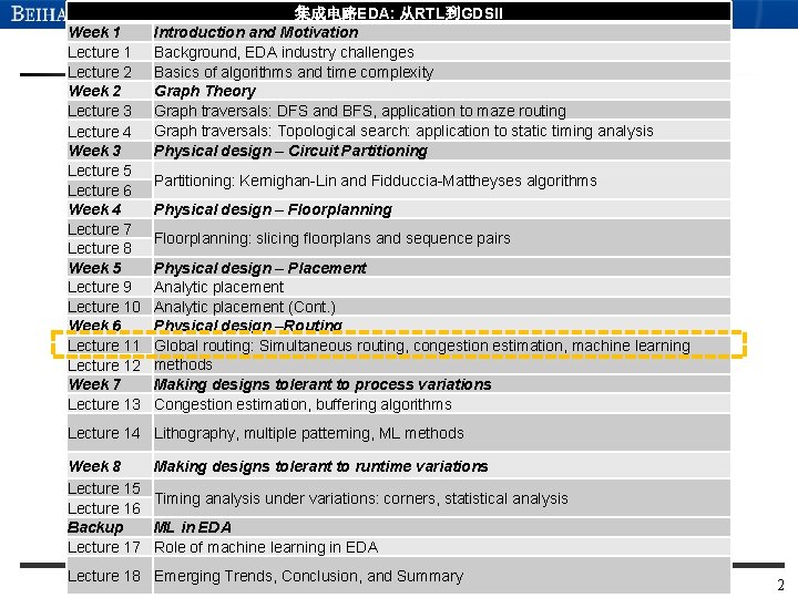
Week 1 Lecture 2 Week 2 Lecture 3 Lecture 4 Week 3 Lecture 5 Lecture 6 Week 4 Lecture 7 Lecture 8 Week 5 Lecture 9 Lecture 10 Week 6 Lecture 11 Lecture 12 Week 7 Lecture 13 集成电路EDA: 从RTL到GDSII Introduction and Motivation Background, EDA industry challenges Basics of algorithms and time complexity Graph Theory Graph traversals: DFS and BFS, application to maze routing Graph traversals: Topological search: application to static timing analysis Physical design – Circuit Partitioning: Kernighan-Lin and Fidduccia-Mattheyses algorithms Physical design – Floorplanning: slicing floorplans and sequence pairs Physical design – Placement Analytic placement (Cont. ) Physical design –Routing Global routing: Simultaneous routing, congestion estimation, machine learning methods Making designs tolerant to process variations Congestion estimation, buffering algorithms Lecture 14 Lithography, multiple patterning, ML methods Week 8 Lecture 15 Lecture 16 Backup Lecture 17 Making designs tolerant to runtime variations Timing analysis under variations: corners, statistical analysis ML in EDA Role of machine learning in EDA Lecture 18 Emerging Trends, Conclusion, and Summary 2

Routing I

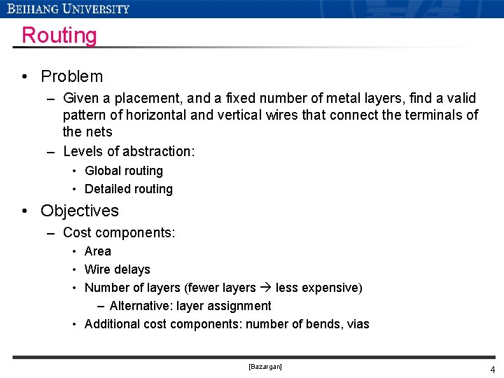
Routing • Problem – Given a placement, and a fixed number of metal layers, find a valid pattern of horizontal and vertical wires that connect the terminals of the nets – Levels of abstraction: • Global routing • Detailed routing • Objectives – Cost components: • Area • Wire delays • Number of layers (fewer layers less expensive) – Alternative: layer assignment • Additional cost components: number of bends, vias [Bazargan] 4

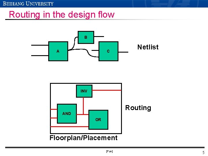
Routing in the design flow B A C Netlist INV Routing AND OR Floorplan/Placement [Pan] 5

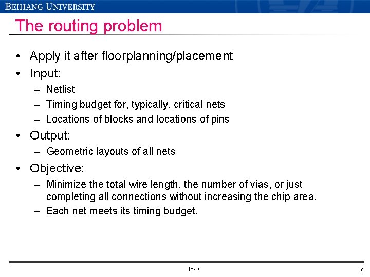
The routing problem • Apply it after floorplanning/placement • Input: – Netlist – Timing budget for, typically, critical nets – Locations of blocks and locations of pins • Output: – Geometric layouts of all nets • Objective: – Minimize the total wire length, the number of vias, or just completing all connections without increasing the chip area. – Each net meets its timing budget. [Pan] 6

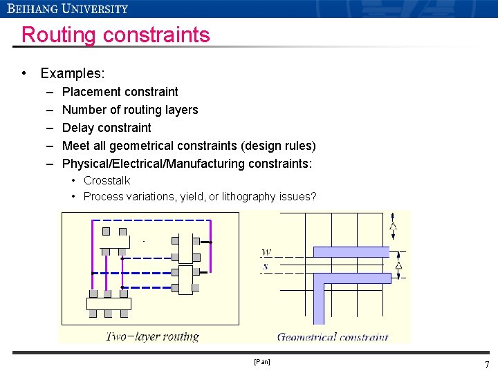
Routing constraints • Examples: – – – Placement constraint Number of routing layers Delay constraint Meet all geometrical constraints (design rules) Physical/Electrical/Manufacturing constraints: • Crosstalk • Process variations, yield, or lithography issues? [Pan] 7

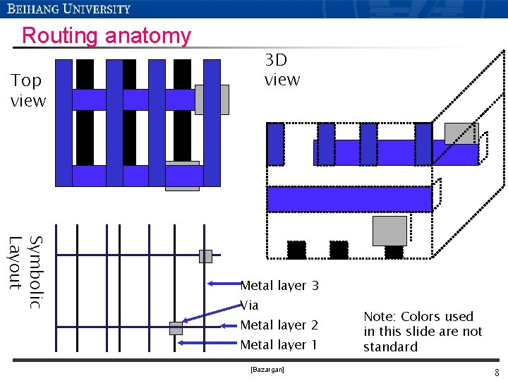
Routing anatomy 3 D view Top view Symbolic Layout Metal layer 3 Via Metal layer 2 Metal layer 1 [Bazargan] Note: Colors used in this slide are not standard 8

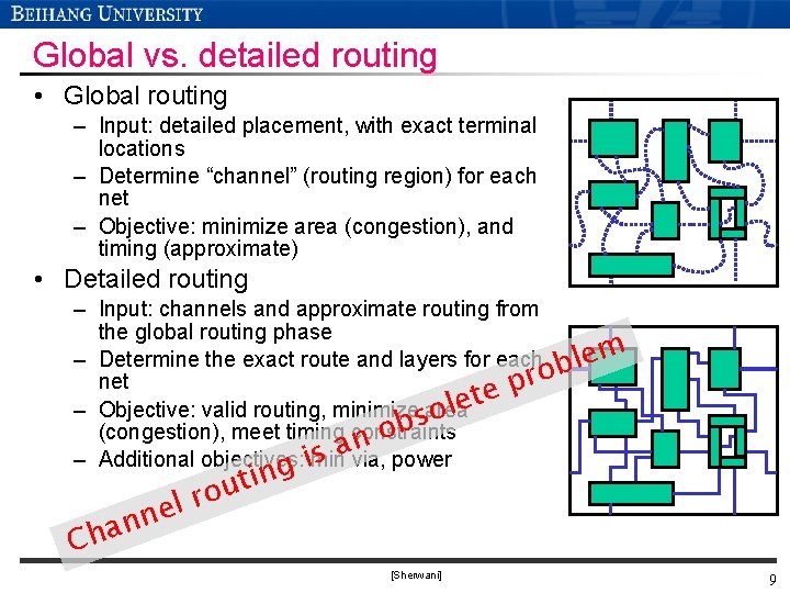
Global vs. detailed routing • Global routing – Input: detailed placement, with exact terminal locations – Determine “channel” (routing region) for each net – Objective: minimize area (congestion), and timing (approximate) • Detailed routing – Input: channels and approximate routing from the global routing phase – Determine the exact route and layers for each blem ro net p e t e l – Objective: valid routing, minimizesarea o b (congestion), meet timing constraints o n a s via, power – Additional objectives: g imin l e n n a h C in t u ro [Sherwani] 9

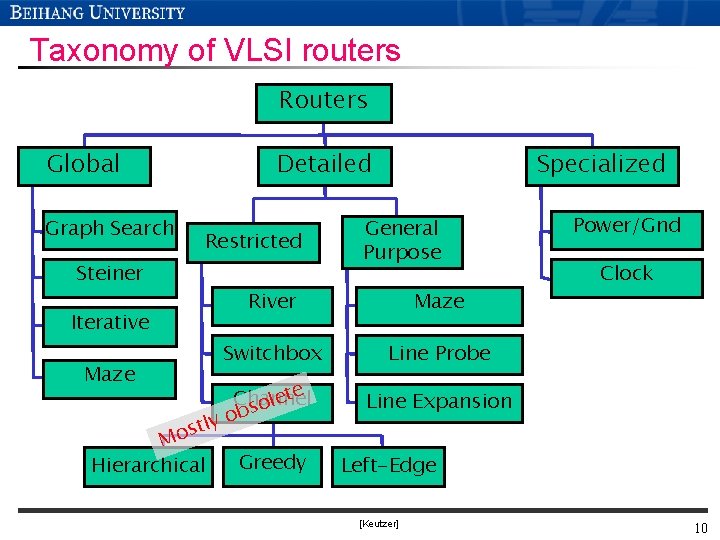
Taxonomy of VLSI routers Routers Global Graph Search Detailed Restricted Steiner Iterative Maze st Mo Hierarchical Specialized General Purpose River Maze Switchbox Line Probe te e Channel l o s b o ly Greedy Power/Gnd Clock Line Expansion Left-Edge [Keutzer] 10

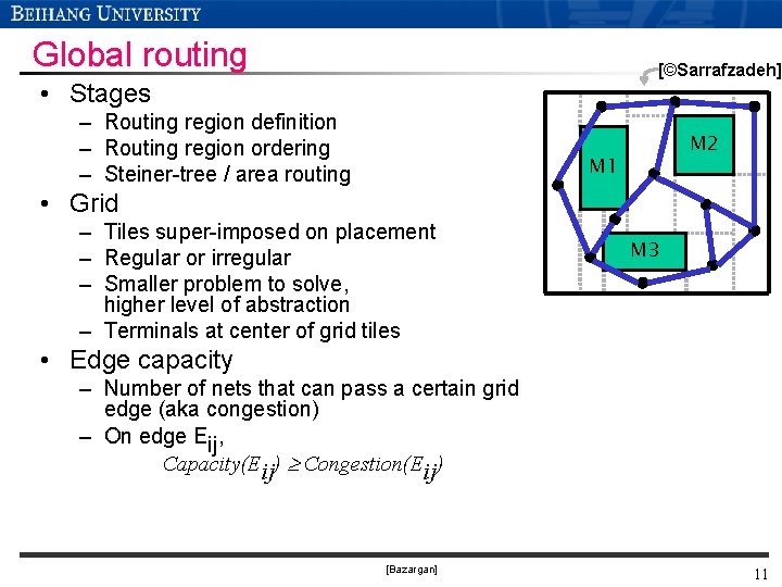
Global routing [©Sarrafzadeh] • Stages – Routing region definition – Routing region ordering – Steiner-tree / area routing M 2 M 1 • Grid – Tiles super-imposed on placement – Regular or irregular – Smaller problem to solve, higher level of abstraction – Terminals at center of grid tiles M 3 • Edge capacity – Number of nets that can pass a certain grid edge (aka congestion) – On edge Eij, Capacity(Eij) Congestion(Eij) [Bazargan] 11

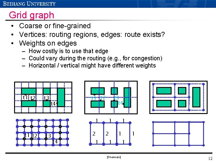
Grid graph • Coarse or fine-grained • Vertices: routing regions, edges: route exists? • Weights on edges – How costly is to use that edge – Could vary during the routing (e. g. , for congestion) – Horizontal / vertical might have different weights t 1 t 2 t 3 t 4 t 1 t 2 t 3 t 4 2 1 t 3 t 4 1 2 1 1 1 [Sherwani] 1 1 12

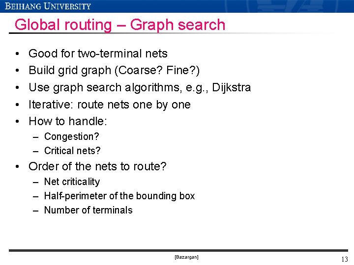
Global routing – Graph search • • • Good for two-terminal nets Build grid graph (Coarse? Fine? ) Use graph search algorithms, e. g. , Dijkstra Iterative: route nets one by one How to handle: – Congestion? – Critical nets? • Order of the nets to route? – Net criticality – Half-perimeter of the bounding box – Number of terminals [Bazargan] 13

Maze routing [Pan]

The maze routing problem • Given: – A planar rectangular grid graph. – Two points S and T on the graph. – Obstacles modeled as blocked vertices. • Objective: – Find the shortest path connecting S and T. • This technique can be used in global or detailed routing (switchbox) problems. [Pan] 15

Grid graph S S S ü T Area Routing X X T Grid Graph (Maze) [Pan] X X ü ü T Simplified Representation 16

Maze routing S T [Pan] 17

Lee’s algorithm: Basic idea • “An Algorithm for Path Connection and its Application”, C. Y. Lee, IRE Transactions on Electronic Computers, 1961. • A Breadth-First Search (BFS) of the grid graph. • Always finds the shortest path possible. • Consists of two phases: – Wave Propagation – Retrace [Pan] 18

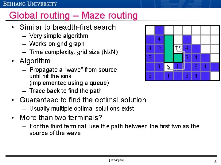
Global routing – Maze routing • Similar to breadth-first search – Very simple algorithm – Works on grid graph – Time complexity: grid size (Nx. N) • Algorithm – Propagate a “wave” from source until hit the sink (implemented using a queue) – Trace back to find the path 5 5 4 4 3 3 2 2 1 3 2 t 5 s 1 5 4 5 3 4 5 1 2 3 4 5 5 • Guaranteed to find the optimal solution – Usually multiple optimal solutions exist • More than two terminals? – For the third terminal, use the path between the first two as the source of the wave [Bazargan] 19

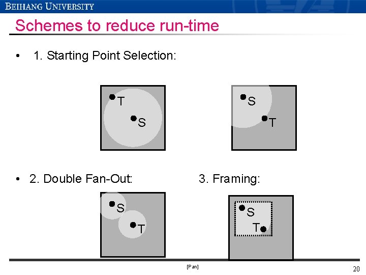
Schemes to reduce run-time • 1. Starting Point Selection: T S S T • 2. Double Fan-Out: 3. Framing: S S T T [Pan] 20

Multi-terminal nets • For a k-terminal net, connect the k terminals using a rectilinear Steiner tree with the shortest wire length on the maze. • This problem is NP-Complete. • Just want to find some good heuristics. [Pan] 21

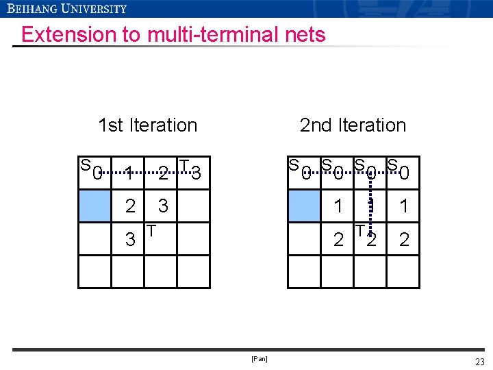
Multi-terminal nets • This problem can be solved by extending the Lee’s algorithm: – Connect one terminal at a time, or – Search for several targets simultaneously, or – Propagate wave fronts from several different sources simultaneously. [Pan] 22

Extension to multi-terminal nets 1 st Iteration S 0 1 2 T 3 2 3 3 2 nd Iteration S 0 S 0 1 T 2 [Pan] T 1 1 2 2 23

Maze routing • Key to popularity: – Simplicity – Guaranteed to find the optimal solution – Can realize more complex cost functions too (e. g. , number of bends in a path) • Weakness: – Multiple terminals not handled efficiently – Dependent on grid, a two dimensional data structure • Different variations exist – Soukup’s alg: • First use DFS, when get to an obstacle, use BFS to get around • No guarantee to find the shortest path [Bazargan] 24

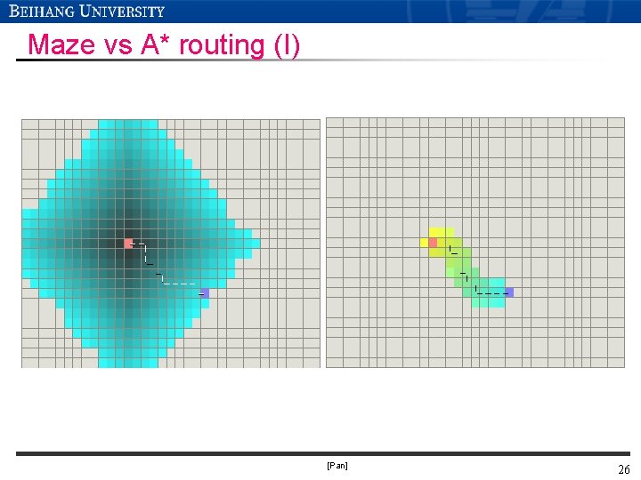
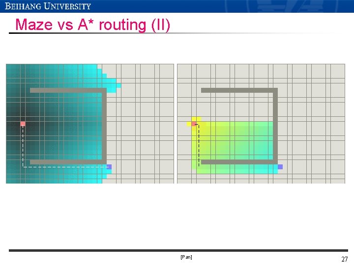
BFS based maze routing (A*) • Need to search whole space? – Guide the search to the goal explicitly • A* search is faster if you need “good path”, not “perfect path” – Use priority queue – C(n) = F(n)+H(n) • F(n) is a computed cost from source to current location. • H(n) is a predicted cost from current location to target. • If H(n)=0, it becomes maze routing! – Optimal (shortest path) when H(n) <= H’(n) (no overestimation) • H’(n) is the exact cost • H(n)=0 never overestimates! [Pan] 25

Maze vs A* routing (I) [Pan] 26

Maze vs A* routing (II) [Pan] 27

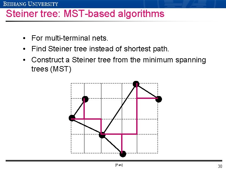
Multi-terminal nets: Steiner trees • Steiner tree (aka Rectilinear Steiner Tree – RST): – A tree connecting multiple terminals • Original points: “demand points” – set D • Added points: “Steiner points” – set S – Edges horizontal or vertical only • Steiner Minimum Tree (SMT) – Similar to minimum spanning tree (MST) – But finding SMT is NP-complete – Many good heuristics introduced to find SMT • Algorithm – Find MST – Pass horizontal and vertical lines from each terminal to get the Hannan grid (optimal solution is on this grid) – Convert each edge of the MST to an L-shaped route on Hanan grid (add a Steiner point at the corner of L) [Bazargan] 28

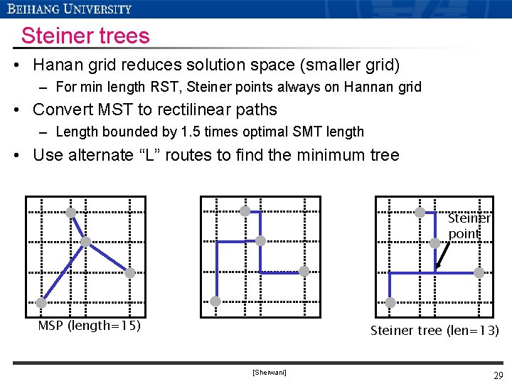
Steiner trees • Hanan grid reduces solution space (smaller grid) – For min length RST, Steiner points always on Hannan grid • Convert MST to rectilinear paths – Length bounded by 1. 5 times optimal SMT length • Use alternate “L” routes to find the minimum tree Steiner point MSP (length=15) Steiner tree (len=13) [Sherwani] 29

Steiner tree: MST-based algorithms • For multi-terminal nets. • Find Steiner tree instead of shortest path. • Construct a Steiner tree from the minimum spanning trees (MST) [Pan] 30

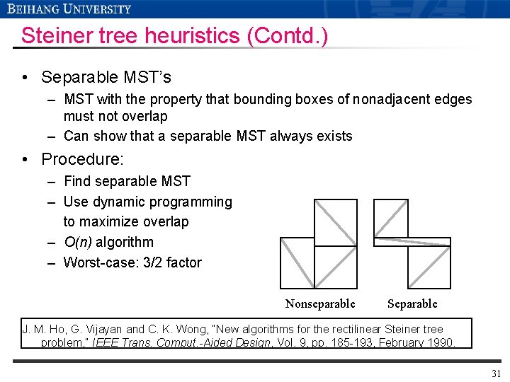
Steiner tree heuristics (Contd. ) • Separable MST’s – MST with the property that bounding boxes of nonadjacent edges must not overlap – Can show that a separable MST always exists • Procedure: – Find separable MST – Use dynamic programming to maximize overlap – O(n) algorithm – Worst-case: 3/2 factor Nonseparable Separable J. M. Ho, G. Vijayan and C. K. Wong, “New algorithms for the rectilinear Steiner tree problem, ” IEEE Trans. Comput. -Aided Design, Vol. 9, pp. 185 -193, February 1990. 31

Steiner tree routing • Can apply different costs to different regions (or horizontal/vertical preference) • Order of the nets – Sequential • Use # of terminals, criticality, etc. to determine order – Parallel • Divide the chip into large regions, perform the routing in parallel • Key to popularity – Fast (not theoretically, but practically) – Bounded solution quality • Shortcomings – Difficult to predict or avoid congestion [Bazargan] 32

Steiner tree heuristics • Iterated 1 -Steiner heuristic – (Not based on MST/SMT ratio) – In each iteration, add one Steiner point • • Consider all O(n 2) candidate Steiner points Construct MST’s for each one and choose the mincost point Cost = O(n 2) O(n log n) = O(n 3 log n) per 1 -Steiner point Number of Steiner points = O(n) – Alternative approach (Georgakopoulous/Papadimitriou) • O(n 2) cost per 1 -Steiner point – Performance: within a factor of 4/3 of optimal for Steiner trees that are “unions of pluses” (instead of 3/2) For details of proofs, see A. B. Kahng and G. Robins, On Optimal Interconnections for VLSI, Kluwer Academic Publishers, 1995, and references therein. 33

Global routing approaches • A combination of different approaches might be used in chip-level routing – Route simple nets (2 -3 pins in local area) directly (e. g. , L-shaped or Z-shaped) – Use “close to optimal” Steiner Tree algorithms to route nets of intermediate length – Route remaining “big” nets using a maze router • Ordering – Some ordering is chosen, if can route all, then done, otherwise: – Rip-up and Re-route [Keutzer] 34

Motivation • Can now build a global route for a single net • Problem – Actual routing cost depends on other nets (congestion, criticality, etc. ) – Possibilities • Route the nets one by one - suboptimal • Route them simultaneously – Ideal algorithm: optimal – Real algorithm that works in a reasonable time: not guaranteed optimal, but “less suboptimal” than routing the nets one by one 35

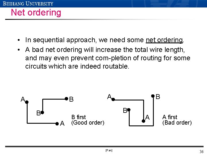
Net ordering • In sequential approach, we need some net ordering. • A bad net ordering will increase the total wire length, and may even prevent com-pletion of routing for some circuits which are indeed routable. A B B A A B B B first (Good order) [Pan] A A first (Bad order) 36

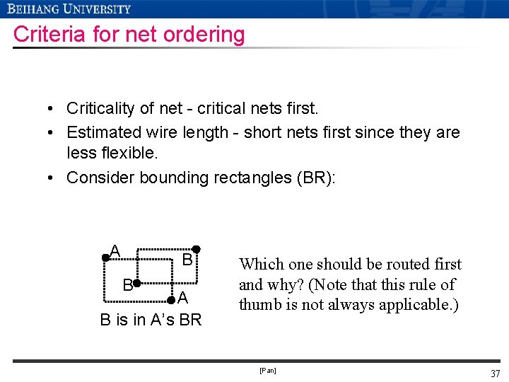
Criteria for net ordering • Criticality of net - critical nets first. • Estimated wire length - short nets first since they are less flexible. • Consider bounding rectangles (BR): A B B A B is in A’s BR Which one should be routed first and why? (Note that this rule of thumb is not always applicable. ) [Pan] 37

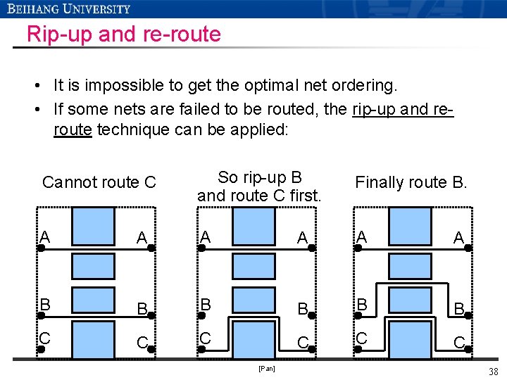
Rip-up and re-route • It is impossible to get the optimal net ordering. • If some nets are failed to be routed, the rip-up and reroute technique can be applied: Cannot route C So rip-up B and route C first. Finally route B. A A A B B B C C C [Pan] 38

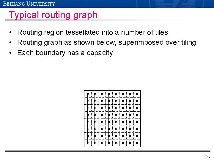
Typical routing graph • Routing region tessellated into a number of tiles • Routing graph as shown below, superimposed over tiling • Each boundary has a capacity 39

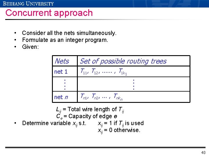
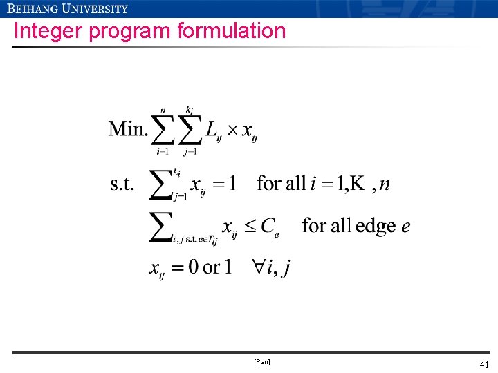
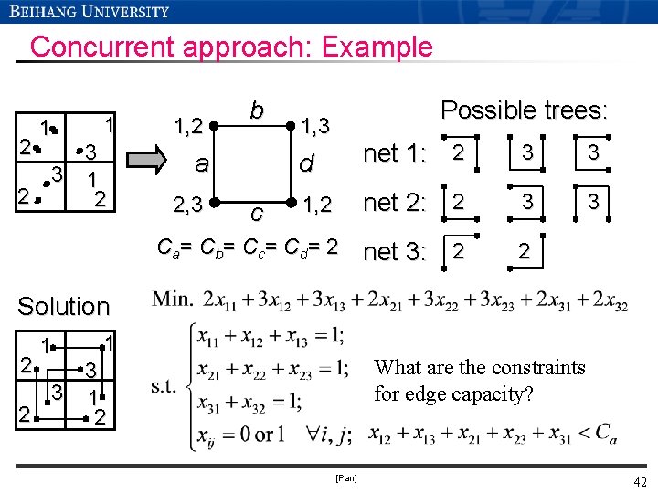
Concurrent approach • Consider all the nets simultaneously. • Formulate as an integer program. • Given: Nets Set of possible routing trees net 1 T 11, T 12, . . . , T 1 k 1 : : net n : : Tn 1, Tn 2, . . . , Tnkn Lij = Total wire length of Tij Ce = Capacity of edge e • Determine variable xij s. t. xij = 1 if Tij is used xij = 0 otherwise. 40

Integer program formulation [Pan] 41

Concurrent approach: Example 2 1 1 3 3 1 2 2 1, 2 b a 2, 3 c Possible trees: 1, 3 d net 1: 2 3 3 1, 2 net 2: 2 3 3 net 3: 2 2 Ca= Cb= Cc= Cd= 2 Solution 2 1 1 What are the constraints for edge capacity? 3 3 1 2 2 [Pan] 42

Integer programming approach · · Standard techniques to solve IP. No net ordering. Give global optimum. Can be extremely slow, especially for large problems. To make it faster, a fewer choices of routing trees for each net can be used. May make the problem infeasible or give a bad solution. · Determining a good set of choices of routing trees is a hard problem by itself. [Pan] 43