Interpolation and Extrapolation Motivation Motivation Table occupancy in

Interpolation and Extrapolation.

Motivation:

Motivation. Table occupancy in a restaurant. Time of day

Modeling of trends CDC data:

Approximate a shape:

Engineering tools of yore for drawing smooth curves.
 that")
Two broad problems to address: • Problem one: Run a continuous line (curve) that goes through each of the give data point exactly. (``connect the dots”). • Problem Two: Fit the existing data in a ``best” way that shows the trend. Trend line.

Example of a “linear fit” to data.
 that goes")
Two problems to address: • Problem one: Run a continuous line (curve) that goes through each of the give data point exactly. (``connect the dots”). • Problem Two: Fit the existing data in a ``best” way that shows the trend. Trend line. Makes sense if no error in the data points. No “noise”. need an exact fit.

Polynomials. Simple & Easy.
 • 2. Polynomial of order n.")
Polynomial interpolation • 1. Linear (connect the dots) • 2. Polynomial of order n. There always exists a polynomial of order at most n-1 that runs through each point in the table.

Constructing an interpolating polynomial. Newtons’ form. Good for recursive programming.
")
Interpolating polynomial. Newton’s form. • An example: P(x)

Possible use for polynomial interpolation. • Represent a smooth shape with a polynomial?

How many sample points needed to “decently” approximate a curve with a polynomial? • Enough to capture the curve’s mins and maxs. • Or enough to capture its roots. • Example: 3 roots, need a polynomial of degree 3

For many functions, a polynomial interpolation can be very accurate

Polynomial interpolation works in many cases, but not always.

A very simple function to interpolate

Polynomial Approximation Weierstrass Approximation Theorem. Suppose f is a continuous realvalued function defined on the real interval [a, b]. For every ε > 0, there exists a polynomial p such that for all x in [a, b], we have | f (x) − p(x)| < ε. Which means you can approximate any continuous function as accurately as you want, by a polynomial. Note: nothing is said about the nodes being equidistant. Opens the possibility of using more complex, non-equidistant placing of the nodes for an accurate approximation. Compare to previously mentioned upper bound on the accuracy. Note 2: nothing is said about the degree of the polynomial, or whether it has to pass exactly through a and b.

Spline Interpolation

What about realistic shape modeling?

Autodesk design:

General definitions •
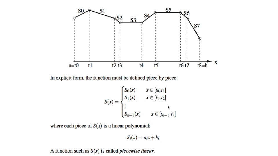
 spline •")
Second degree (quadratic) spline •

An example •

An example •

Cubic spline •

An example: •

An example: •
 – spline defined on knots tn Y = Y(t)")
Parametric splines: X = X(t) – spline defined on knots tn Y = Y(t) – spline defined on knots tn t 2 Control points t 1

Power point “curve” function. • “right click” to edit points. • “Local” effect of tweaking each control point.
 Global. BSpline. Surface. Interpolation. cdf")
Splines in 3 D (A Mathematica example available) Global. BSpline. Surface. Interpolation. cdf

Polynomials are, generally, a bad idea for functions that do not look like polynomials.

A few fixes still exist, they may improve things, but only go so far. • (*Fix 1. Increase n*)(*Rarely works. Generally BAD idea*) • (*Fix 2. Extend range of data. May approximates well if region of interest is deep inside the new range*) • (*Fix 3. “Best”: use non-uniform or "unequally spaced" control/data points e. g. Chebyshev points: xi=cos[Pi*(2 i+1)/(2 n+2)], i[Less. Equal]n*)(*data=Table[N[{0. 5*((a+b)+ b-a)*Cos[(i/n)*Pi]), F[0. 5*((a+b)+(b-a)*Cos[(i/n)*Pi])]}], {i, 0, n}]*)

But, the best idea is to choose a more appropriate model • Fix 4. Use more appropriate MODEL (basis functions). Gaussian in OUR case of the bell-shaped spread of data points. fit=Fit[data, Table[Exp[-i*1. 0*x^2], {i, 1, n}], x]
 that goes")
Two problems to address: • Problem one: Run a continuous line (curve) that goes through each of the give data point exactly. (``connect the dots”). • Problem Two: Fit the existing data in a ``best” way that shows the trend. Trend line.
- Slides: 37