6 2 Interpolation and Extrapolation Interpolation is a

6. 2 Interpolation and Extrapolation • Interpolation is a method of new data points from a discrete set of knows data points. • In Physics Obtained a number of data points by sampling or some experiment, and tries to construct a function which closely fit these data points. This is called curve fitting. Interpolation is a specific case of curve fitting We sometimes know the value of a function f(x) at a set of points x 1, x 2, …, x. N, but we don’t have an analytic expression for f(x) that lets us calculate its value at an arbitrary point. For example the f(x)’s result from some physical measurement that can be cast into a simple function form.

If the desired x is in between the largest and smallest of the x’s, the problem is called interpolation; if x is outside the range it is called extrapolation. Interpolation process has two stages: Fit an interpolation function to the data points provided. Evaluate that interpolation function at the target point x. The number of points used in an interpolation scheme is called the order of the interpolation. Increasing the order does not necessarily increase the accuracy, especially in polynomial interpolation.

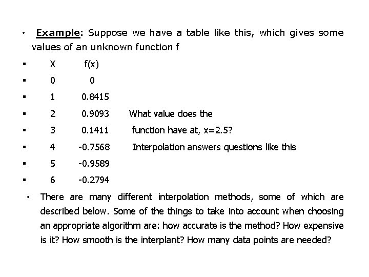
Example: Suppose we have a table like this, which gives some • values of an unknown function f X f(x) 0 0 1 0. 8415 2 0. 9093 3 0. 1411 4 -0. 7568 5 -0. 9589 6 -0. 2794 • What value does the function have at, x=2. 5? Interpolation answers questions like this There are many different interpolation methods, some of which are described below. Some of the things to take into account when choosing an appropriate algorithm are: how accurate is the method? How expensive is it? How smooth is the interplant? How many data points are needed?

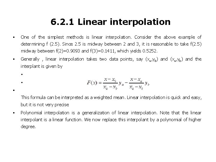
6. 2. 1 Linear interpolation One of the simplest methods is linear interpolation. Consider the above example of determining f (2. 5). Since 2. 5 is midway between 2 and 3, it is reasonable to take f(2. 5) midway between f(2)=0. 9093 and f(3)=0. 1411, which yields 0. 5252. Generally , linear interpolation takes two data points, say (xa, yb) and the interplant is given by • • This formula can be interpreted as a weighted mean. Linear interpolation is quick and easy, but it is not very precise Polynomial interpolation is a generalization of linear interpolation. Note that the linear interpolant is a linear function. We now replace this interpolant by a polynomial of higher degree.

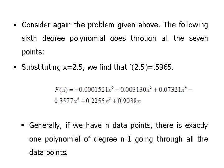
Consider again the problem given above. The following sixth degree polynomial goes through all the seven points: Substituting x=2. 5, we find that f(2. 5)=. 5965. Generally, if we have n data points, there is exactly one polynomial of degree n-1 going through all the data points.

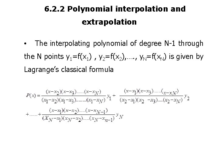
6. 2. 2 Polynomial interpolation and extrapolation • The interpolating polynomial of degree N-1 through the N points y 1=f(x 1) , y 2=f(x 2), …. , y. N=f(x. N) is given by Lagrange’s classical formula

• There are N terms , each a polynomial of degree N-1. • Let p 1 be the value at x of the unique polynomial of degree zero passing through the point (x 1, y 1); so p 1=y 1. Also, define p 2, p 3, . . , p. N. • Now, let p 12 be the value at x of the unique polynomial of degree one passing through both(x 1, y 1)and(x 2, y 2). Likewise p 23, p 34, . . , p(N-1)N. • Similarly, for higher-order, up to p 123…. N, which is the value of the unique interpolating polynomial through all N points?

• The computational procedure used in computer software for the evaluation of a library function such as sin(x), Cos(x) or ex involves polynomial approximation. Suppose that the function f(x) =ex is to be approximated by a polynomial of degree n=2 over the interval [ -1, 1]. The Taylor approximation p(x) =1. 0+1. 0 x+0. 5 x 2. • An associated problem involves the construction of the collection polynomial. Given n+1 points in the plane, the collection polynomial is the unique polynomial of degree ≤ n which passes through the points. • For example, the collection polynomial of degree n=4 that passes through the five points (1, 2), (2, 1), (3, 5), (4, 6) and (5, 1) is: • P(x)=[504 - 806 x + 427 x 2 - 82 x 3 + 5 x 4]/24

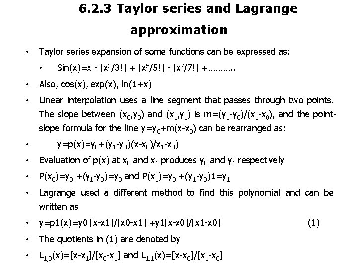
6. 2. 3 Taylor series and Lagrange approximation • Taylor series expansion of some functions can be expressed as: • Sin(x)=x - [x 3/3!] + [x 5/5!] - [x 7/7!] +………. . • Also, cos(x), exp(x), ln(1+x) • Linear interpolation uses a line segment that passes through two points. The slope between (x 0, y 0) and (x 1, y 1) is m=(y 1 -y 0)/(x 1 -x 0), and the pointslope formula for the line y=y 0+m(x-x 0) can be rearranged as: • y=p(x)=y 0+(y 1 -y 0)(x-x 0)/x 1 -x 0) • Evaluation of p(x) at x 0 and x 1 produces y 0 and y 1 respectively • P(x 0)=y 0 +(y 1 -y 0)=y 0 and P(x 1)=y 0 +(y 1 -y 0)1=y 1 • Lagrange used a different method to find this polynomial and can be written as • y=p 1(x)=y 0 [x-x 1]/[x 0 -x 1] +y 1[x-x 0]/[x 1 -x 0] • The quotients in (1) are denoted by • L 1, 0(x)=[x-x 1]/[x 0 -x 1] and L 1, 1(x)=[x-x 0]/[x 1 -x 0] (1)

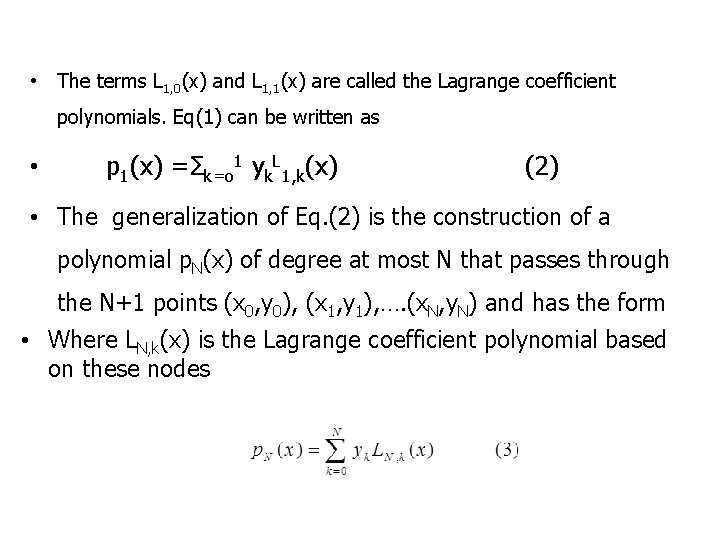
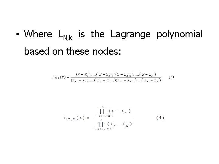
• The terms L 1, 0(x) and L 1, 1(x) are called the Lagrange coefficient polynomials. Eq(1) can be written as • p 1(x) =Σk=o 1 yk. L 1, k(x) (2) • The generalization of Eq. (2) is the construction of a polynomial p. N(x) of degree at most N that passes through the N+1 points (x 0, y 0), (x 1, y 1), …. (x. N, y. N) and has the form • Where LN, k(x) is the Lagrange coefficient polynomial based on these nodes

• Where LN, k is the Lagrange polynomial based on these nodes:

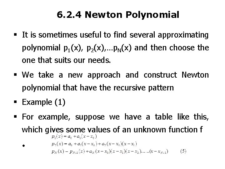
6. 2. 4 Newton Polynomial It is sometimes useful to find several approximating polynomial p 1(x), p 2(x), …p. N(x) and then choose the one that suits our needs. We take a new approach and construct Newton polynomial that have the recursive pattern Example (1) For example, suppose we have a table like this, which gives some values of an unknown function f •

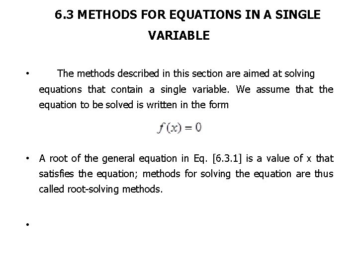
6. 3 METHODS FOR EQUATIONS IN A SINGLE VARIABLE • The methods described in this section are aimed at solving equations that contain a single variable. We assume that the equation to be solved is written in the form • A root of the general equation in Eq. [6. 3. 1] is a value of x that satisfies the equation; methods for solving the equation are thus called root-solving methods. •

6. 3. 1 The incremental-Search method • The incremental-search method is a numerical analog of finding a root of Eq. [6. 3. 1] by plotting f(x) versus x to see where f (x) crosses the x axis. The procedure is as follows. • • Procedure of incremental-search method: 1. Set a counter I to zero, choose a starting value x 0, choose an increment h, and compute a reference value f 0, equal to f (x 0). • 2. Increase I by 1, set xi equal to (x 0 + ih), and compute f(xi). • 3. If {f 0 [f(xi)]}>0, return to Step 2; otherwise, go on to Step 4. • 4. Estimate the root x from: x = xi – h [f(xi)]/[ f(xi)- f(xi-h)].

• The idea in procedure 6. 3. 1 is to begin at a starting point x 0 and search along the x axis in the increments h until we find two successive points (xi – h) and xi whose line segment contains a root. This segment is indicated when the function first becomes zero or changes sign; that is, when the product [f 0 f(xi)] first becomes less than or equal to zero. The root is then estimated by linear interpolation in Step 4. • The magnitude of the increment h represents a crude error bound for the estimated solution because it is the length of the segment on which the exact solution lies. The sign of h dictates the search direction from the starting point x 0. If no solution exists in that direction, the method will obviously fail. The number of iterations should be limited to prevent infinite looping in such an instance. Failure and infinite looping can also occur when h is large in magnitude and the equation has two closely spaced roots. If the line segment from (xi-h) to xi contains both roots, the function values at the search points would have the same sign. The test of Step 3 would then fail to indicate the presence of the roots. • Another condition that may cause failure is a discontinuity. Consider for example, the function

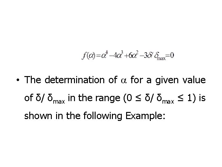
• The function is discontinuous when x is equal to 1. It tends to (-∞) as x approaches 1 from above, and it tends to (+∞) as x approaches 1 from below. Application of incremental search procedure to solving f(x) = 0 could cause the existence of a root to be falsely indicated when two search points lie on the opposite sides of (x = 1). • To illustrate the incremental search method, we consider the deflection of a horizontal cantilevered beam when it is subjected to a uniform, vertical load. Abeam extending from its clamped end (x = 0) to its free end (x = L) has a maximum deflection δmax at (x = L). The deflection δ at the location (x = a. L) is related to δmax by

• The determination of a for a given value of δ/ δmax in the range (0 ≤ δ/ δmax ≤ 1) is shown in the following Example: