Inner Tracker Alignment study Kim Vervink Monday seminar

Inner Tracker Alignment study Kim Vervink Monday seminar, 10 th April 2006, EPFL 10. 04. 2006 K. Vervink

Overview • General alignment strategy • Mechanical point of view: – limits on assembly precision and metrology • First Inner Tracker misalignment study: effect of a misaligned detector on the pattern recognition performance • Selection of high quality track sample for alignment • Introduction to Millepede: theory – Theory – Constraints – Generation of tracks and geometry • Testing of Millepede Toy Mc – straight line tracks • Different degrees of freedom • Dependencies – Parabola’s • Conclusion 10. 04. 2006 K. Vervink 2

Alignment strategy 1. Precise module assembly (closest as possible to design values) 2. System metrology to provide an initial set of alignment constants (next slides) 3. Online fast alignment method (Internal and global)* In full discussion mode (alignment workshop, lots of philosophical discussions) 4. Offline alignment monitoring to ensure track quality during data taking Status: Velo is far advanced (implementation in Gaudi) IT & OT toy study level Alignment Strategy should be determined by September 2006 Here presented IT standalone internal alignment with the millepede method. Toy MC with generation of detector geometry and tracks. Sensitivity test (to dof) not a speed test 10. 04. 2006 K. Vervink 3

Mechanical side: how well can offsets be measured mechanically? Goal: precise knowledge of where the ith strip is within the LHCb coordinates (not the position but the knowledge of the position is important) Ladder level: where is sensor on ladder (assembly precision 50 mm) Precise measurements Single and double? Ladder in Box: Strategy of measuring not defined yet. Plexiglas box? Hand machined!! Cover plate with inserts where the pilars are placed Box on frame expected values less then 0. 5 mm but if the survey group can’t measure from inside the magnet the precision could be around 3 mm. 10. 04. 2006 Cover plate: honneycomb + CF sandwich Reasonably stable, but this is no Alu or Steel K. Vervink 4

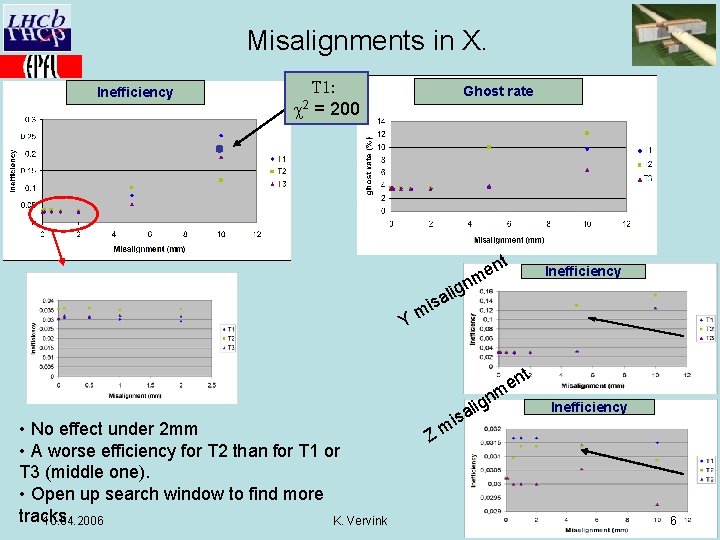
Misalignment pre-study Goal: how well works the pattern recognition with a misaligned detector? How many tracks are made by a wrong asignment of hits? Check this with existing track finding algorithms (TSA and general one): * written to give an optimum result in a perfect aligned detector. * Track acception depends on a c 2 cut between the measurement points and track fit. * One could play around with this value to obtain the optimum c 2 cut for finding tracks with a misaligned detector. Method: Tracking Seeding Algorithm (uses only IT hits) move one by one the 3 IT stations in different directions. Study the effect on: – ghost rate, – inefficiency of the track finding algorithm – Comparison with the general pat. Rec (uses also OT hits) Extra: preparation of a selection of a sample of clean tracks that will be used for 10. 04. 2006 K. Vervink 5 alignment of IT

Misalignments in X. Inefficiency T 1: c 2 = 200 Ghost rate t en m ign Inefficiency l Y sa mi t l en m ign • No effect under 2 mm • A worse efficiency for T 2 than for T 1 or T 3 (middle one). • Open up search window to find more tracks 10. 04. 2006 K. Vervink Z sa i m Inefficiency 6

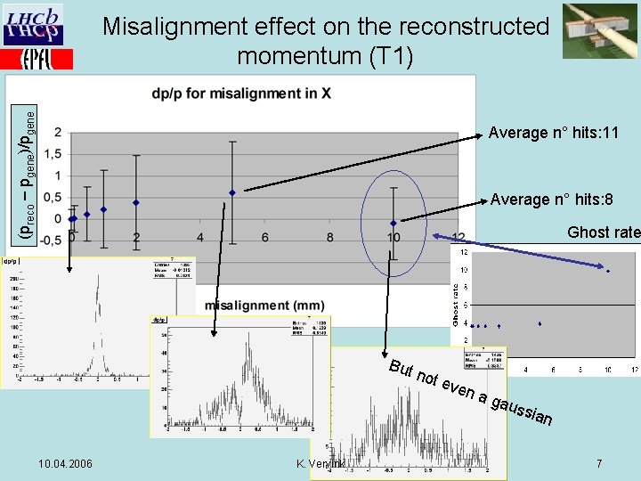
(preco – pgene)/pgene Misalignment effect on the reconstructed momentum (T 1) Average n° hits: 11 Average n° hits: 8 Ghost rate But 10. 04. 2006 K. Vervink not eve n a ga uss ian 7

Comparison of pat. recognition algorithms Standard tracking algorithm: -Loses efficiency sooner -Runs over the whole T station (=75% more tracks) this explains why the inefficiency settles at 25%, which means no IT tracks were taken into account. Only shapes are comparable, not values! 10. 04. 2006 K. Vervink 8

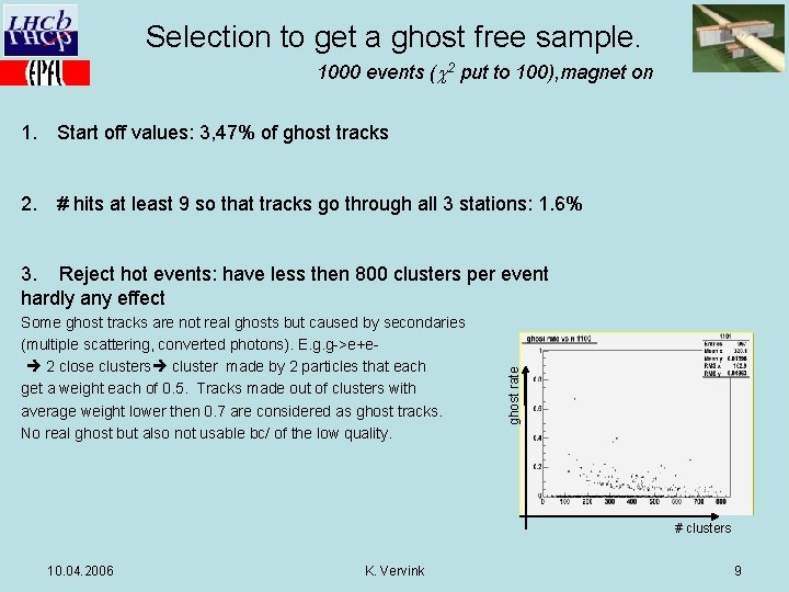
Selection to get a ghost free sample. 1000 events (c 2 put to 100), magnet on 1. Start off values: 3, 47% of ghost tracks 2. # hits at least 9 so that tracks go through all 3 stations: 1. 6% Some ghost tracks are not real ghosts but caused by secondaries (multiple scattering, converted photons). E. g. g->e+e 2 close clusters cluster made by 2 particles that each get a weight each of 0. 5. Tracks made out of clusters with average weight lower then 0. 7 are considered as ghost tracks. No real ghost but also not usable bc/ of the low quality. ghost rate 3. Reject hot events: have less then 800 clusters per event hardly any effect # clusters 10. 04. 2006 K. Vervink 9

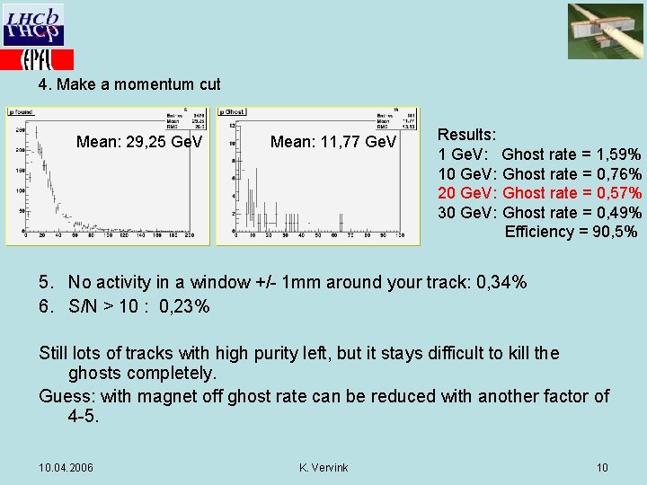
4. Make a momentum cut Mean: 29, 25 Ge. V Mean: 11, 77 Ge. V Results: 1 Ge. V: Ghost rate = 1, 59% 10 Ge. V: Ghost rate = 0, 76% 20 Ge. V: Ghost rate = 0, 57% 30 Ge. V: Ghost rate = 0, 49% Efficiency = 90, 5% 5. No activity in a window +/- 1 mm around your track: 0, 34% 6. S/N > 10 : 0, 23% Still lots of tracks with high purity left, but it stays difficult to kill the ghosts completely. Guess: with magnet off ghost rate can be reduced with another factor of 4 -5. 10. 04. 2006 K. Vervink 10

Introduction to the alignment strategy Classical alignment method: minimizing residuals r xtrue Using the track fit (several planes): xmeas r = alignment parameter = difference between fitted and measured value. Not a correct method because your track fit is a results of wrong measurements. The result will be biased. Better to fit simultaneous the track parameters (local parameters) and alignment parameters (global parameters). This is done by expressing the alignment offsets in a linear function of the local derivatives (1, z) 10. 04. 2006 K. Vervink 11

In general your equation looks like this (misalignemts in x and y) j: the track parameters are different per track, but the same for every plane i: the offsets and measurements and z positions are the same for each track but different for each plane The measurement depends on the track and plane How to simulate measurements on stereo-angles: work with u and v measurements instead of x and y (in reality you just get a umeas. ) For x work as well with u and v but the stereo angles are then 0° 10. 04. 2006 K. Vervink 12

Degrees of freedom that make the problem non-linear: Dz, Dg Problem becomes non-linear: the track model includes terms where alignment parameters are multiplied by other alignment parameters and track parameters Expand in Taylor series and keep only linear terms in misalignment corrections. 10. 04. 2006 K. Vervink x Y Dz a. Dz c. Dz g y. Dg -x. Dg 13

Overview of the local and global derivatives for all 6 degrees of freedom DOF Global on x part Global on y part x -Dx - y - -Dy z a Dz c. Dz a a y Da c y Da b a x Db c x Db g y Dg -x Dg : parameters that have to be obtained from the measurement approximate Local parameters for straight line tracks: 1, z parabolic tracks: 1, z, z 2 10. 04. 2006 K. Vervink 14

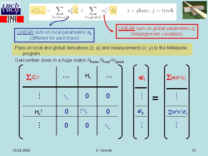
LINEAR sum on global parameters Dil (misalignment constants) LINEAR sum on local parameters ajk (different for each track) Pass on local and global derivatives (z, D) and measurements (x, y) to the Millepede program. Gets written down in a huge matrix Ntracks. Nlocal+Nglobal 0 0 0 K. Vervink ajk = wkxi, jzik … 0 0 … 0 Gi, jk wlxi, j. Dil ajl … … 10. 04. 2006 Hk … … Hk T … … l. Cli, j 15

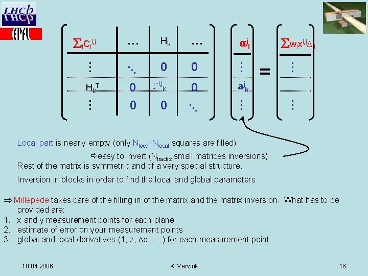
0 Gi, jk 0 ajk … 0 0 0 = … 0 wlxi, j. Dil ajl … … Hk T … … l. Cli, j Local part is nearly empty (only Nlocal∙Nlocal squares are filled) ðeasy to invert (Ntracks small matrices inversions) Rest of the matrix is symmetric and of a very special structure. Inversion in blocks in order to find the local and global parameters Millepede takes care of the filling in of the matrix and the matrix inversion. What has to be provided are: 1. x and y measurement points for each plane 2. estimate of error on your measurement points 3. global and local derivatives (1, z, Dx, …. ) for each measurement point 10. 04. 2006 K. Vervink 16

Constraints It is very important that the correct constraints are given as well in a form that can be included in the matrix (with Lagrange multiplier method): In function of the global parameters (not of the local!) i: plane Principle: constraint (for each dof) due to freedom that can slip into the local parameter. x = a +bz + cz 2 Shearing and scaling Translation, rotation 10. 04. 2006 K. Vervink 17

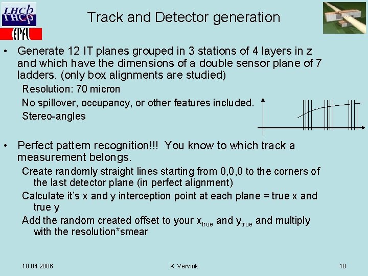
Track and Detector generation • Generate 12 IT planes grouped in 3 stations of 4 layers in z and which have the dimensions of a double sensor plane of 7 ladders. (only box alignments are studied) Resolution: 70 micron No spillover, occupancy, or other features included. Stereo-angles • Perfect pattern recognition!!! You know to which track a measurement belongs. Create randomly straight lines starting from 0, 0, 0 to the corners of the last detector plane (in perfect alignment) Calculate it’s x and y interception point at each plane = true x and true y Add the random created offset to your xtrue and ytrue and multiply with the resolution*smear 10. 04. 2006 K. Vervink 18

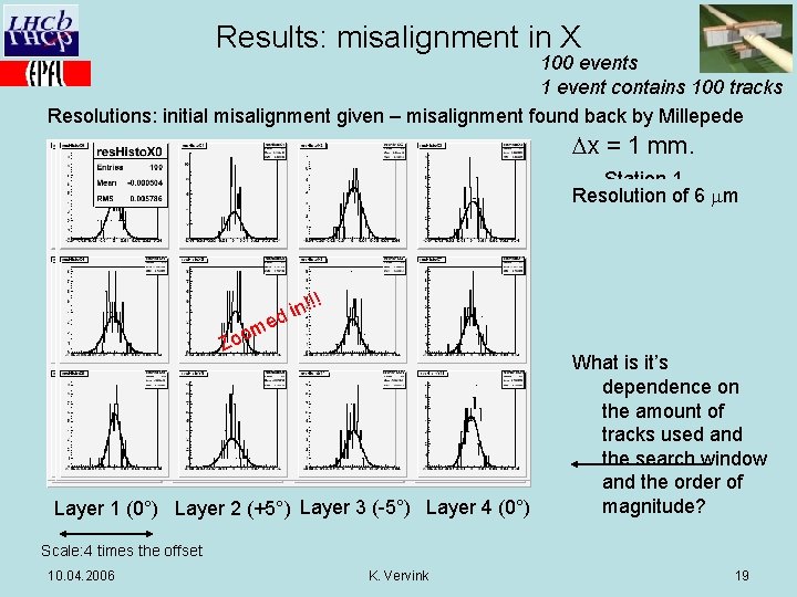
Results: misalignment in X 100 events 1 event contains 100 tracks Resolutions: initial misalignment given – misalignment found back by Millepede Dx = 1 mm. Station 1 Resolution of 6 mm ! Station 2 me o Zo !! n i d Layer 1 (0°) Layer 2 (+5°) Layer 3 (-5°) Layer 4 (0°) What is it’s dependence on the amount of Station 3 tracks used and the search window and the order of magnitude? Scale: 4 times the offset 10. 04. 2006 K. Vervink 19

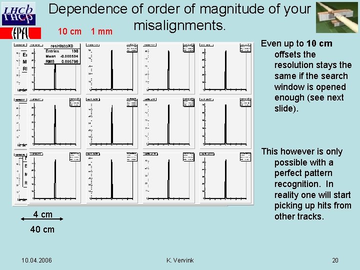
Dependence of order of magnitude of your misalignments. 10 cm 1 mm Even up to 10 cm offsets the resolution stays the same if the search window is opened enough (see next slide). This however is only possible with a perfect pattern recognition. In reality one will start picking up hits from other tracks. 4 cm 40 cm 10. 04. 2006 K. Vervink 20

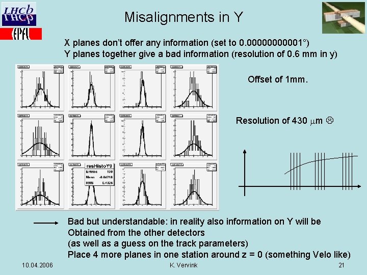
Misalignments in Y X planes don’t offer any information (set to 0. 000001°) Y planes together give a bad information (resolution of 0. 6 mm in y) Offset of 1 mm. Resolution of 430 mm Bad but understandable: in reality also information on Y will be Obtained from the other detectors (as well as a guess on the track parameters) Place 4 more planes in one station around z = 0 (something Velo like) 10. 04. 2006 K. Vervink 21

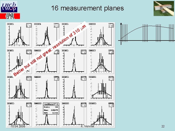
16 measurement planes o es e n till er t t Be 10. 04. 2006 r tg r : t a of n o uti m m 0 31 l o ts u b K. Vervink 22

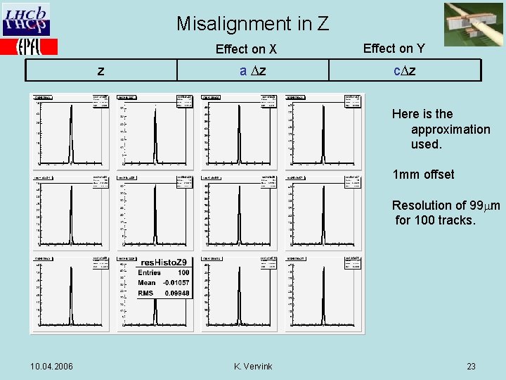
Misalignment in Z Effect on X z a Dz Effect on Y c. Dz Here is the approximation used. 1 mm offset Resolution of 99 mm for 100 tracks. 10. 04. 2006 K. Vervink 23

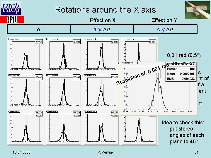
Rotations around the X axis a Effect on X Effect on Y a y Da c y Da 0, 01 rad (0. 5°) : of n o i lut o Res rad 4 0 0. 0 Very bad results: Highly dependent of the quality of a y measurement Basically one measurement per station Idea to check this: put stereo angles of each plane to 45° 10. 04. 2006 K. Vervink 24

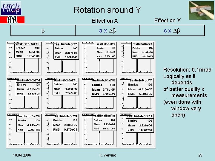
Rotation around Y Effect on X b a x Db Effect on Y c x Db Resolution: 0, 1 mrad Logically as it depends of better quality x measurements (even done with window very open) 10. 04. 2006 K. Vervink 25

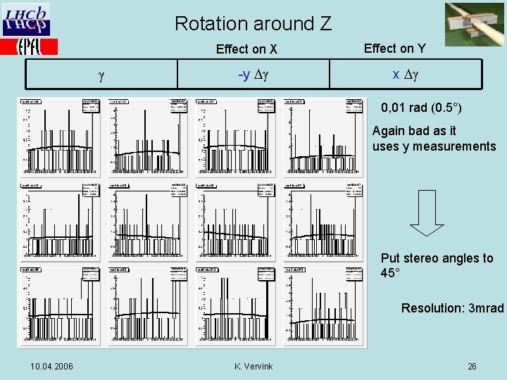
Rotation around Z Effect on X g -y Dg Effect on Y x Dg 0, 01 rad (0. 5°) Again bad as it uses y measurements Put stereo angles to 45° Resolution: 3 mrad 10. 04. 2006 K. Vervink 26

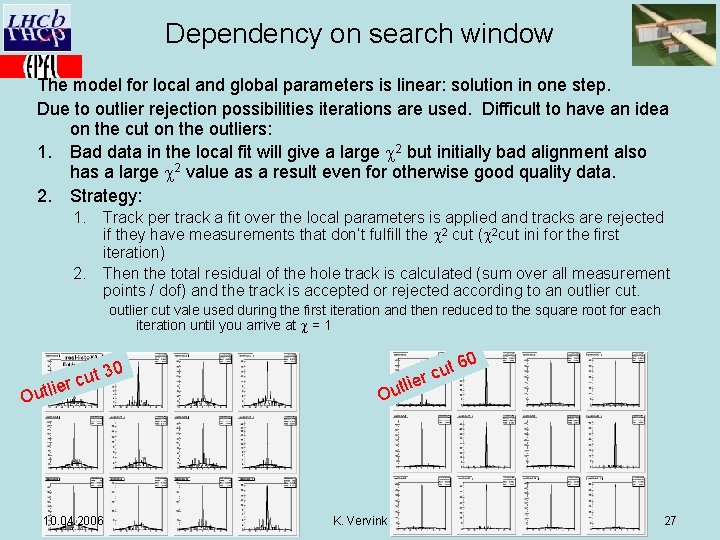
Dependency on search window The model for local and global parameters is linear: solution in one step. Due to outlier rejection possibilities iterations are used. Difficult to have an idea on the cut on the outliers: 1. Bad data in the local fit will give a large c 2 but initially bad alignment also has a large c 2 value as a result even for otherwise good quality data. 2. Strategy: 1. Track per track a fit over the local parameters is applied and tracks are rejected if they have measurements that don’t fulfill the c 2 cut (c 2 cut ini for the first iteration) 2. Then the total residual of the hole track is calculated (sum over all measurement points / dof) and the track is accepted or rejected according to an outlier cut vale used during the first iteration and then reduced to the square root for each iteration until you arrive at c = 1 r ie Outl 0 cut 3 10. 04. 2006 0 t 6 u c r utlie O K. Vervink 27

The direct solution: without iterations! This strategy can be meaningful only if the global parameters represent only a small correction to the fit and a cut based on residuals of the local fits is meaningful (= 3 st. dev) 10. 04. 2006 K. Vervink 28

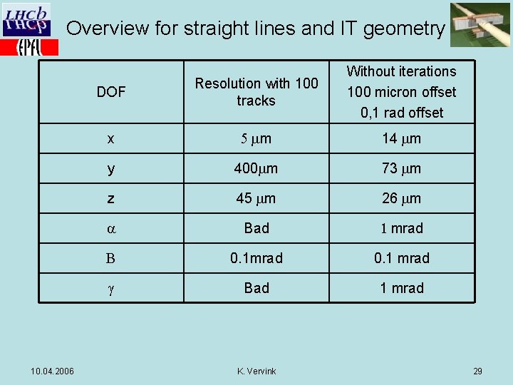
Overview for straight lines and IT geometry 10. 04. 2006 DOF Resolution with 100 tracks Without iterations 100 micron offset 0, 1 rad offset x 5 mm 14 mm y 400 mm 73 mm z 45 mm 26 mm a Bad 1 mrad B 0. 1 mrad 0. 1 mrad g Bad 1 mrad K. Vervink 29

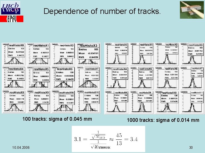
Dependence of number of tracks. 100 tracks: sigma of 0. 045 mm 10. 04. 2006 1000 tracks: sigma of 0. 014 mm K. Vervink 30

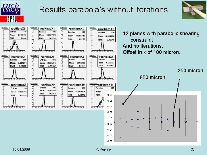
Parabolic tracks Local derivatives become 1, z and z 2 Extra constraint: parabolic shearing: Lots of trouble with this: even with more planes and with the parabolic shearing included, different resolutions per plane 3 stations of 4 layers is not enough to find a good resolution (basically only 3 measurements) Try without iterations and offsets in x of 100 micron (no clue why it doesn’t work with iterations, also lots of tracks don’t pass the selection) and equidistant planes. 10. 04. 2006 K. Vervink 31

Results parabola’s without iterations 12 planes with parabolic shearing constraint And no iterations. Offset in x of 100 micron. 250 micron 650 micron 10. 04. 2006 K. Vervink 32

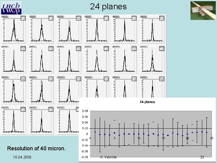
24 planes Resolution of 40 micron. 10. 04. 2006 K. Vervink 33

Conclusion and outlook Pre-study on the pattern recognition showed a stable behavior of the efficiency with the current algorithm up until 2 mm. Ghost rate can be reduced until 0. 2% but not killed completely Standalone IT alignment with perfect pattern recognition shows for straight line tracks a resolution of 10 mm in x. Still not everything understood for parabola’s and iterations To do (not by me anymore) Prepare Millepede for “testbeam” on one box (started) Study use of overlaps between 4 boxes in one station, how to find misalignments between ladders, … Write things down. Continue to understand Millepede with parabola’s (Florin) 10. 04. 2006 K. Vervink 34