Informed search algorithms Chapter 4 Outline n n

Informed search algorithms Chapter 4

Outline n n n n n Best-first search Greedy best-first search A* search Heuristics Local search algorithms Hill-climbing search Simulated annealing search Local beam search Genetic algorithms

Best-first search n Idea: use an evaluation function f(n) for each node n n n f(n) provides an estimate for the total cost. Expand the node n with smallest f(n). Implementation: Order the nodes in fringe increasing order of cost. Special cases: n n greedy best-first search A* search

Romania with straight-line dist.

Greedy best-first search n n n f(n) = estimate of cost from n to goal e. g. , f(n) = straight-line distance from n to Bucharest Greedy best-first search expands the node that appears to be closest to goal.

Greedy best-first search example

Greedy best-first search example

Greedy best-first search example

Greedy best-first search example

Properties of greedy best-first search Think of an example n n Complete? No – can get stuck in loops. Time? O(bm), but a good heuristic can give dramatic improvement Space? O(bm) - keeps all nodes in memory Optimal? No e. g. Arad Sibiu Rimnicu Virea Pitesti Bucharest is shorter!

A* search n n n n Idea: avoid expanding paths that are already expensive Evaluation function f(n) = g(n) + h(n) g(n) = cost so far to reach n h(n) = estimated cost from n to goal f(n) = estimated total cost of path through n to goal Best First search has f(n)=h(n) Uniform Cost search has f(n)=g(n)

Admissible heuristics n n A heuristic h(n) is admissible if for every node n, h(n) ≤ h*(n), where h*(n) is the true cost to reach the goal state from n. An admissible heuristic never overestimates the cost to reach the goal, i. e. , it is optimistic Example: h. SLD(n) (never overestimates the actual road distance) Theorem: If h(n) is admissible, A* using TREESEARCH is optimal

A* search example

* A search example

A* search example

A* search example

A* search example

A* search example

Properties of A* n n Complete? Yes (unless there are infinitely many nodes with f ≤ f(G) , i. e. step-cost > ε) Time/Space? Exponential except if: Optimal? Yes Optimally Efficient: Yes (no algorithm with the same heuristic is guaranteed to expand fewer nodes)

Optimality of A* (proof) n Suppose some suboptimal goal G 2 has been generated and is in the fringe. Let n be an unexpanded node in the fringe such that n is on a shortest path to an optimal goal G. We want to prove: f(n) < f(G 2) (then A* will prefer n over G 2) n f(G 2) = g(G 2) f(G) = g(G) g(G 2) > g(G) since h(G 2) = 0 since h(G) = 0 since G 2 is suboptimal n f(G 2) > f(G) from above h(n) g(n) + h(n) f(n) ≤ ≤ ≤ < n n n h*(n) g(n) + h*(n) f(G 2) since h is admissible (under-estimate) from above since g(n)+h(n)=f(n) & g(n)+h*(n)=f(G) from

Consistent heuristics n A heuristic is consistent if for every node n, every successor n' of n generated by any action a, h(n) ≤ c(n, a, n') + h(n') n If h is consistent, we have f(n’) n n = = ≥ ≥ g(n’) + h(n’) g(n) + c(n, a, n') + h(n’) g(n) + h(n) = f(n) (by def. ) (g(n’)=g(n)+c(n. a. n’)) (consistency) i. e. , f(n) is non-decreasing along any path. It’s the triangle inequality ! keeps all checked nodes in memory to avoid repeated Theorem: If h(n) is consistent, A* using GRAPH-SEARCH is optimal states

Optimality of A* n n n A* expands nodes in order of increasing f value Gradually adds "f-contours" of nodes Contour i contains all nodes with f≤fi where fi < fi+1

A 3 S 2 B 6 4 1 C D straight-line distances 1 F 8 E 20 1 G h(S-G)=10 h(A-G)=7 h(D-G)=1 h(F-G)=1 h(B-G)=10 h(E-G)=8 h(C-G)=20 try yourself The graph above shows the step-costs for different paths going from the start (S) to the goal (G). On the right you find the straight-line distances. 1. Draw the search tree for this problem. Avoid repeated states. 2. Give the order in which the tree is searched (e. g. S-C-B. . . -G) for A* search. Use the straight-line dist. as a heuristic function, i. e. h=SLD, and indicate for each node visited what the value for the evaluation function, f, is.

Memory Bounded Heuristic Search: Recursive BFS n n n How can we solve the memory problem for A* search? Idea: Try something like depth first search, but let’s not forget everything about the branches we have partially explored. We remember the best f-value we have found so far in the branch we are deleting.

RBFS: best alternative over fringe nodes, which are not children: do I want to back up? RBFS changes its mind very often in practice. This is because the f=g+h become more accurate (less optimistic) as we approach the goal. Hence, higher level nodes have smaller f-values and will be explored first. Problem: We should keep in memory whatever we can.

Simple Memory Bounded A* n n n This is like A*, but when memory is full we delete the worst node (largest f-value). Like RBFS, we remember the best descendent in the branch we delete. If there is a tie (equal f-values) we delete the oldest nodes first. simple-MBA* finds the optimal reachable solution given the memory constraint. A Solution is not reachable if a single path from root to goal does not fit into memory Time can still be exponential.

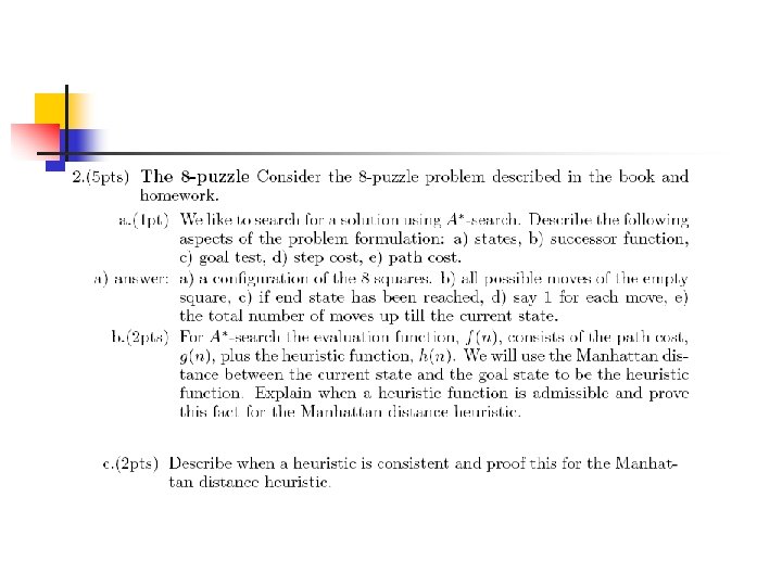
Admissible heuristics E. g. , for the 8 -puzzle: n h 1(n) = number of misplaced tiles n h 2(n) = total Manhattan distance (i. e. , no. of squares from desired location of each tile) n n h 1(S) = ? h 2(S) = ?

Admissible heuristics E. g. , for the 8 -puzzle: n h 1(n) = number of misplaced tiles n h 2(n) = total Manhattan distance (i. e. , no. of squares from desired location of each tile) n n h 1(S) = ? 8 h 2(S) = ? 3+1+2+2+2+3+3+2 = 18

Dominance n n n If h 2(n) ≥ h 1(n) for all n (both admissible) then h 2 dominates h 1 h 2 is better for search: it is guaranteed to expand less or equal nr of nodes. n Typical search costs (average number of nodes expanded): n d=12 n d=24 IDS = A*(h 1) A*(h 2) 3, 644, 035 nodes = 227 nodes = 73 nodes too many nodes = 39, 135 nodes = 1, 641 nodes

Relaxed problems n n A problem with fewer restrictions on the actions is called a relaxed problem The cost of an optimal solution to a relaxed problem is an admissible heuristic for the original problem If the rules of the 8 -puzzle are relaxed so that a tile can move anywhere, then h 1(n) gives the shortest solution If the rules are relaxed so that a tile can move to any adjacent square, then h 2(n) gives the shortest solution

Local search algorithms n n n In many optimization problems, the path to the goal is irrelevant; the goal state itself is the solution State space = set of "complete" configurations Find configuration satisfying constraints, e. g. , nqueens In such cases, we can use local search algorithms keep a single "current" state, try to improve it. Very memory efficient (only remember current state)

Example: n-queens n Put n queens on an n × n board with no two queens on the same row, column, or diagonal Note that a state cannot be an incomplete configuration with m<n queens

Hill-climbing search n Problem: depending on initial state, can get stuck in local maxima

Gradient Descent • Assume we have some cost-function: and we want minimize over continuous variables X 1, X 2, . . , Xn 1. Compute the gradient : 2. Take a small step downhill in the direction of the gradient: 3. Check if 4. If true then accept move, if not reject. 5. Repeat.

Exercise • Describe the gradient descent algorithm for the cost function:

Hill-climbing search: 8 -queens problem Each number indicates h if we move a queen in its corresponding column n h = number of pairs of queens that are attacking each other, either directly or indirectly (h = 17 for the above state)

Hill-climbing search: 8 -queens problem n A local minimum with h = 1 what can you do to get out of this local minima? )

Simulated annealing search n n Idea: escape local maxima by allowing some "bad" moves but gradually decrease their frequency. This is like smoothing the cost landscape.

Properties of simulated annealing search n n One can prove: If T decreases slowly enough, then simulated annealing search will find a global optimum with probability approaching 1 (however, this may take VERY long) Widely used in VLSI layout, airline scheduling, etc.

Local beam search n Keep track of k states rather than just one. n Start with k randomly generated states. n n At each iteration, all the successors of all k states are generated. If any one is a goal state, stop; else select the k best successors from the complete list and repeat.

Genetic algorithms n A successor state is generated by combining two parent states n Start with k randomly generated states (population) n A state is represented as a string over a finite alphabet (often a string of 0 s and 1 s) n Evaluation function (fitness function). Higher values for better states. n Produce the next generation of states by selection, crossover, and mutation

fitness: #non-attacking queens probability of being regenerated in next generation n Fitness function: number of non-attacking pairs of queens (min = 0, max = 8 × 7/2 = 28) P(child) = 24/(24+23+20+11) = 31% P(child) = 23/(24+23+20+11) = 29% etc

Exercise Traveling salesman problem. Given N cities and all their distances, find the shortest tour through all cities. 1. 2. 3. 4. 5. Define representation (genes) Define cross-over (create valid paths) Define mutation Define fitness How do we choose children? DEMO: http: //www-cse. uta. edu/~cook/ai 1/lectures/applets/gatsp/TSP. html

Project Implement a genetic algorithm to solve the following problem: Consider filling a Mx. N rectangle with the numbers 1. . . MN Each number has either 4 neighbors or 3 neighbors (on the edge) or 2 neighbors (in a corner). The total cost is the of all the absolute differences between all neighboring pairs of numbers. We’ll give you a big problem after some deadline and you then have a couple of days to find the best solution you can find. The lowest cost solution wins. 1 5 9 2 6 3 7 4 8 10 11 12 If you come up with a fancy alternative to GA you may request to implement that as an alternative to solve the same problem. cost = |1 -2|+|2 -3|+|3 -4|+|5 -6|+|6 -7|+|7 -8|+|9 -10|+|10 -11|+|11 -12| + |1 -5|+|2 -6|+|3 -7|+|4 -8|+|5 -9|+|6 -10|+|7 -11|+|8 -12|

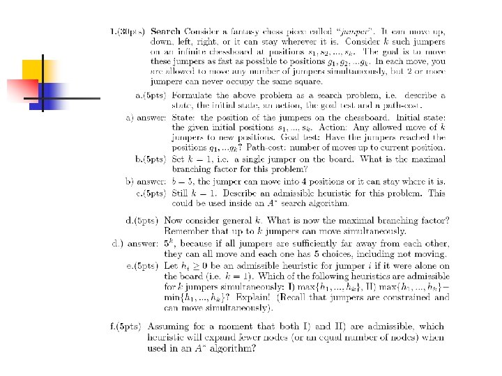
Exercise SEARCH TREE R 9 1) Consider the search tree to the right. There are 2 goal states, G 1 and G 2. The numbers on the edges represent step-costs. You also know the following heuristic estimates: h(B G 2) = 9, h(D G 2)=10, h(A G 1)=2, h(C G 1)=1 a) In what order will A* search visit the nodes? Explain your answer by indicating the value of the evaluation function for those nodes that the algorithm considers. A 1 C 1 G 1 1 B 2 D 10 G 2

3 A 6 D 1 straight-line distances F 1 h(S-G)=10 h(A-G)=7 2 4 8 S G h(D-G)=1 B E h(F-G)=1 h(B-G)=10 1 20 h(E-G)=8 C h(C-G)=20 The graph above shows the step-costs for different paths going from the start (S) to the goal (G). On the right you find the straight-line distances. 1. Draw the search tree for this problem. Avoid repeated states. 2. Give the order in which the tree is searched (e. g. S-C-B. . . -G) for the following search algorithms: a) Breadth-first search, Depth first search, uniform cost search, and A* search. For A* use the straight-line dist. as a heuristic function, i. e. h=SLD, and indicate for each node visited what the value for the evaluation function, f, is. 3. For each algorithm indicate whether it is an informed or an uninformed search strategy. 4. For each algorithm indicate separately whether its time complexity is polynomial or exponential in the number of nodes visited. Same for space complexity. 5. For each algorithm indicate separately whether it is complete and/or optimal. Answer these questions for generic search problems. Assume step-cost positive but not constant, do not assume we can avoid repeated states, do not assume we have a very good heuristic function h.

Appendix n Some details of the MBA* next.

SMA* pseudocode book) (not in 2 nd edition 2 of function SMA*(problem) returns a solution sequence inputs: problem, a problem static: Queue, a queue of nodes ordered by f-cost Queue MAKE-QUEUE({MAKE-NODE(INITIAL-STATE[problem])}) loop do if Queue is empty then return failure n deepest least-f-cost node in Queue if GOAL-TEST(n) then return success s NEXT-SUCCESSOR(n) if s is not a goal and is at maximum depth then f(s) else f(s) MAX(f(n), g(s)+h(s)) if all of n’s successors have been generated then update n’s f-cost and those of its ancestors if necessary if SUCCESSORS(n) all in memory then remove n from Queue if memory is full then delete shallowest, highest-f-cost node in Queue remove it from its parent’s successor list insert its parent on Queue if necessary insert s in Queue end

Simple Memory-bounded A* (SMA*) (Example with 3 -node memory) Progress of SMA*. Each node is labeled with its current f-cost. Values in parentheses show the value of the best forgotten descendant. � = goal 0+12=12 20+5=25 8+5=13 10 C D 16+2=18 E 30+5=35 F 30+0=30 8 J 24+0=24 A A 12 13 G 13 16 H 15 B I 24+0=24 10 A G 8 20+0=20 10 12 8 B 10 A 13[15] A 10 10+5=15 best forgotten node best estimated solution so far for that node Search space f = g+h maximal depth is 3, since memory limit is 3. This branch is now useless. 8 K B G 15 13 A 15[15] A 15[24] A G 15 24[ ] I 24 A 20[24] 8 15 24+5=29 18 H B G 15 24 C B 25 B 20[ ] D Algorithm can tell you when best solution found within memory constraint is optimal or not. 20