Informed Heuristic Search Evaluation Function returns a value

Informed (Heuristic) Search • Evaluation Function returns a value estimating the desirability of expanding a frontier node • Two Basic Approaches – Expand node closest to goal – Expand node on least-cost path to goal • When closest node to goal is always expanded 1 st, its called best first search, or alternately greedy search • How does greedy search differ from uniform cost? • In practice, a heuristic function, called h(n), guesses the cost from the current state to a goal state. • We require: h(n)=0 if n is a goal state.

Greedy Search • Take what looks best right now • Expand node with best h(n) regardless of overall path length • Follows a single path to a solution, backtracks only when a dead end is reached • Increases search speed (problem dependent) BUT – sub-optimal solutions, incompleteness

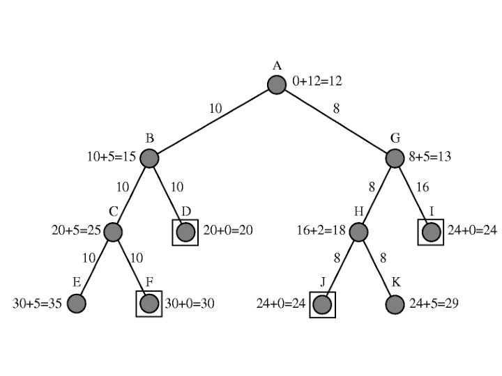
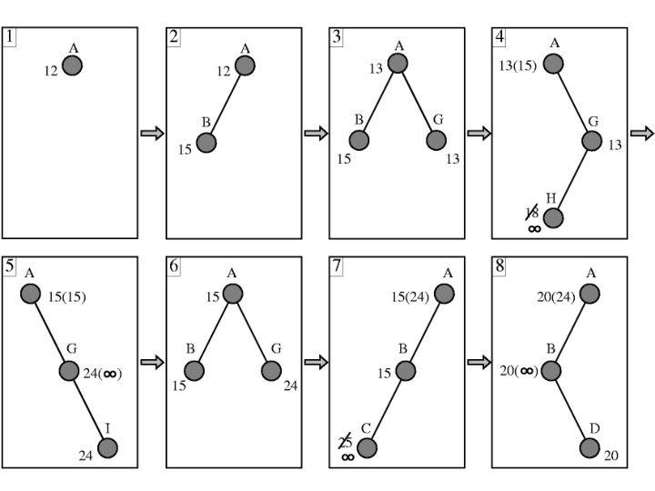
A* Search • Optimal and Complete • To determine next node to expand, Uniform Cost uses g(n), Greedy uses h(n) • A* uses both! f(n) = g(n) + h(n) • f(n) is estimated cost of cheapest solution passing through n. • Hmmm. Is A* optimal?

A* Optimality • A* is optimal if h(n) is admissible • Admissible means it must never overestimate the cost of reaching the goal from n • Is it easy to find admissible heuristics? • Try h(n)=0! (Just uniform cost search)

Heuristics for A* • Usually possible to come up with something (much) better than h(n)=0, i. e. straight line distance for route finding • The closer h(n) is to actual cost, the less search is required to find optimal solution • If you can get h(n) = actual cost, then search proceeds in a straight line to the goal!!! Essentially 0 search!!!

Admissible Heuristics

More on A* Optimality • Definition: f cost never decreases along a path: monotonicity • If h(n) is non-monotonic (unusual) A* is still complete and optimal (if h is admissible) • For any h, can maintain monotonicity and better guess by using pathmax equation: – f(c) = max(f(p), g(c) + h(c)), (where p is parent node and c is a child of p) • A* expands within a growing contour. If f* is cost of optimal solution, then A* expands all nodes with f(n) < f*. Therefore, A* must be optimal • It has been proven that A* is also optimally efficient – In other words, any algorithm that expands less nodes than A* must occasionally produce a non-optimal solution!!!

A* Completeness and Complexity • A* is complete on graphs with finite branching factor where all operators have some MINIMUM positive cost – (very common) • However, in most cases space remains exponential • Search space is sub-exponential only if the error between h and actual cost grows no faster than the log of the actual path cost – |h(n)-h*(n)| <= O(log(h*(n)) • In general h is not this accurate • But we can still save gobs of time and find much better solutions with a good h

Heuristics • The more accurate, the less you explore • Can use inadmissible heuristics, but lose optimality guarantee • Effective branching factor – Like to be close to 1 • Hmm. Can you have a branching factor less than 1?

Comparing Heuristics • How do you determine if h 2 is better than h 1? • For 8 puzzle, let h 1 = # tiles in wrong position, h 2 = Manhattan distance • h 2 dominates h 1 if for all n h 2(n) >= h 1(n) • If h 2 dominates h 1, why is it better? • Guaranteed to expand *no more* and probably less nodes • Must have h 1, h 2 admissible, of course.

Creating Heuristics • Problem specific, but general approach is to look at a relaxed version of the problem – i. e. derive heurstic from the exact cost of a relaxed version of the problem. • H 1 (tile can move anywhere) vs h 2 (tile can move to any adjacent square) for 8 -puzzle • If a problem is formally defined, very easy to produce relaxed versions simply by removing constraints, 1 at a time, until the problem becomes easy enough to calculate exact costs directly.

Choosing Heuristics • • If one dominates all others, use it Otherwise? ? ? use h(n) = max(h 1(n), h 2(n), …) Hmm. Should you also consider the cost of calculating the heuristics? • Could “improve” heuristic by using statistical information on heuristics error • Could use general features of the problem to “create” (or learn) heuristics – checkers example.

Review – differences between? • Uniform Cost? • Greedy? • A* • Which is best?

Complex Problems – IDA* • Often, A* runs out of memory before it runs out of other resources • Use ID for uninformed, IDA* for informed search! • Difference – rather than a depth limit, you use an increasing f-cost limit and do depth first within the contour shaped by the f-cost limit. • Complete, but optimality depends greatly on how you increment the fcost – If too small then you end up restarting iterative deepening after only expanding a few nodes – You MUST expand some reasonable percentage of the frontier, or the cost is ridiculous. – Hmmm. What is the cost if you only expand 1 node every iteration?

SMA* - Simplified Memory Bounded A* • • • Philosophy: Use as much available memory as possible to avoid regeneration problems if IDA* Basic strategy: Use A* algorithm, but when we run out of memory, throw out node with highest f(n) When a node (or subtree) is removed from memory, its ancestor keeps track of the best f-value in that subtree. If later on, the best f-value available in the entire search is higher than that from the “forgotten” subtree, the forgotten node will be regenerated. Not always optimal or complete. Complete only if there is enough memory to store the shallowest solution path. Optimal only if there is enough memory to store the shallowest optimal solution path. SO WHAT? ? !!!? ? ?

• Local search and optimization problems – Hill climbing – Simulated annealing – Genetic algorithms

Optimization Problems

Example: n-queens

Constraint Satisfaction Problems • N-queens is an example of a CSP • World state: well defined set of variables Vi with domain Di • Goal test: satisfy a set of constraints that specify allowable combinations of values for subsets of variables • Depth first search appropriate – path doesn’t matter, only goal state, maximum depth fixed at n, the number of variables, select 1 variable to branch on at each level of the tree

Hill Climbing – Gradient Ascent

Problem – Local Maxima

Simulated Annealing • Gradient Descent style algorithm, but relax the constraint that every change must be an improvement • Start with high temperature (high initial randomness) which allows larger search jumps initially • Allows some random movement which may overcome local minima - randomness a function of how good/bad a particular modification would be • Gradually lower the temperature until system stabilizes • If temp is lowered slowly enough, guaranteed to always produce optimal solution

Simulated Annealing – Basic Algorithm

Genetic Algorithms • GAs are one of the most powerful and applicable search methods available • GA originally developed by John Holland (1975) • Inspired by natural genetics and biological evolution • Uses concept of “survival of fittest” • Genetic operators (crossover, mutation, etc. ) used to modify a pool of state candidates in order to improve them • Survival of the fittest, with reproduction of new possible states coming from best discovered parent states • Iterative procedure (iterative improvement) • Produces a series of “generations of populations” one per iteration • Each member of a population represents a feasible solution, called a chromosome

GA Pseudo Code

X-over Example

GA Pros/Cons • Various Data Representations, One Algorithm • No fancy math involved in the algorithm, however designing an objective can be difficult and confusing • Easy to understand • Works on almost anything – must have objective function • Inherently parallel • Doesn’t work as well as other algorithms in convex (or mostly convex) search spaces – i. e. if you know a smart way to search the space, do it • Depending on complexity, a GA can be computationally expensive • Often requires a lot of tweaking