Chapter 4 Informed Heuristic Search ICS 171 Fall

Chapter 4: Informed Heuristic Search ICS 171 Fall 2006 ICS-171: Notes 4: 1

Summary • Heuristics and Optimal search strategies – heuristics – hill-climbing algorithms – Best-First search – A*: optimal search using heuristics – Properties of A* • admissibility, • monotonicity, • accuracy and dominance • efficiency of A* – Branch and Bound – Iterative deepening A* – Automatic generation of heuristics ICS-171: Notes 4: 2

Problem: finding a Minimum Cost Path • • • Previously we wanted an arbitrary path to a goal or best cost. Now, we want the minimum cost path to a goal G – Cost of a path = sum of individual transitions along path Examples of path-cost: – Navigation • path-cost = distance to node in miles – minimum => minimum time, least fuel – VLSI Design • path-cost = length of wires between chips – minimum => least clock/signal delay – 8 -Puzzle • path-cost = number of pieces moved – minimum => least time to solve the puzzle ICS-171: Notes 4: 3

Best-first search • Idea: use an evaluation function f(n) for each node – estimate of "desirability" Expand most desirable unexpanded node • Implementation: Order the nodes in fringe in decreasing order of desirability • Special cases: – greedy best-first search – A* search ICS-171: Notes 4: 4

Heuristic functions • 8 -puzzle • 8 -queen • Travelling salesperson ICS-171: Notes 4: 5

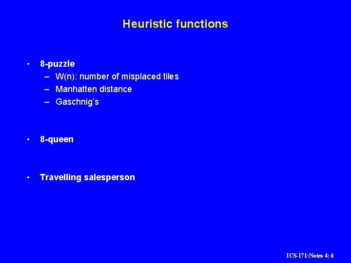
Heuristic functions • 8 -puzzle – W(n): number of misplaced tiles – Manhatten distance – Gaschnig’s • 8 -queen • Travelling salesperson ICS-171: Notes 4: 6

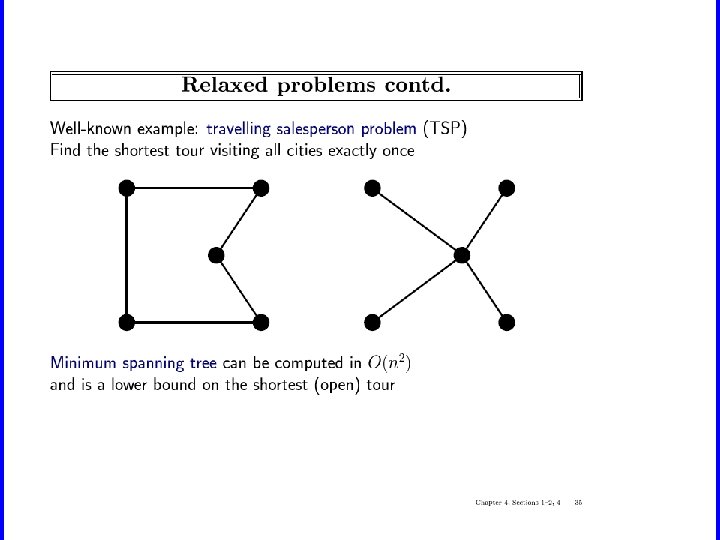
Heuristic functions • 8 -puzzle – W(n): number of misplaced tiles – Manhatten distance – Gaschnig’s • 8 -queen – Number of future feasible slots – Min number of feasible slots in a row • Travelling salesperson – Minimum spanning tree – Minimum assignment problem ICS-171: Notes 4: 7

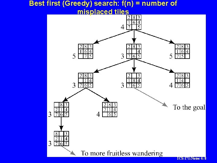
Best first (Greedy) search: f(n) = number of misplaced tiles ICS-171: Notes 4: 8

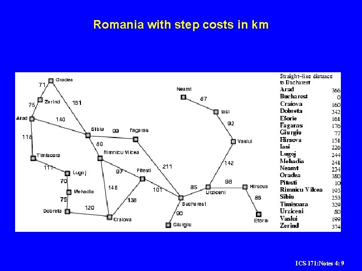
Romania with step costs in km ICS-171: Notes 4: 9

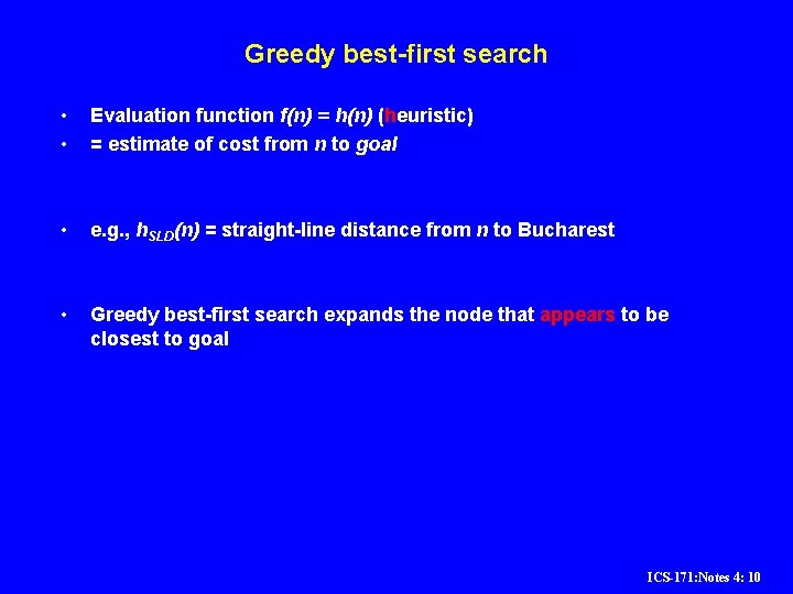
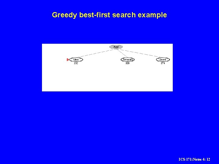
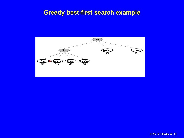
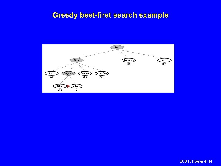
Greedy best-first search • • Evaluation function f(n) = h(n) (heuristic) = estimate of cost from n to goal • e. g. , h. SLD(n) = straight-line distance from n to Bucharest • Greedy best-first search expands the node that appears to be closest to goal ICS-171: Notes 4: 10

Greedy best-first search example ICS-171: Notes 4: 11

Greedy best-first search example ICS-171: Notes 4: 12

Greedy best-first search example ICS-171: Notes 4: 13

Greedy best-first search example ICS-171: Notes 4: 14

Problems with Greedy Search • Not complete • • Get stuck on local minimas and plateaus, Irrevocable, Infinite loops Can we incorporate heuristics in systematic search? ICS-171: Notes 4: 15

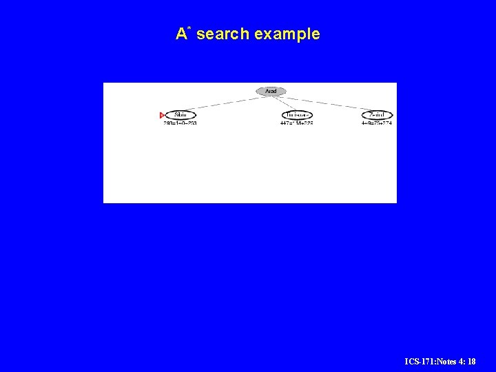
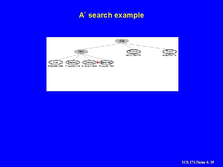
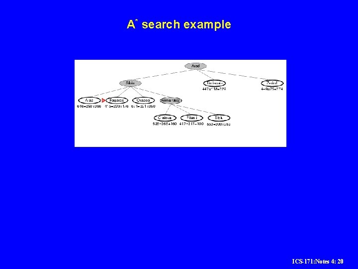
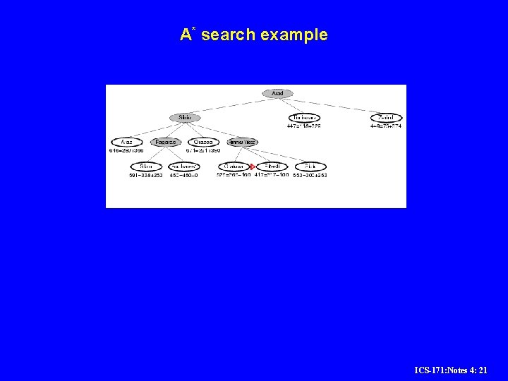
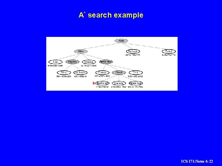
A* search • Idea: avoid expanding paths that are already expensive • Evaluation function f(n) = g(n) + h(n) • g(n) = cost so far to reach n • h(n) = estimated cost from n to goal • f(n) = estimated total cost of path through n to goal ICS-171: Notes 4: 16

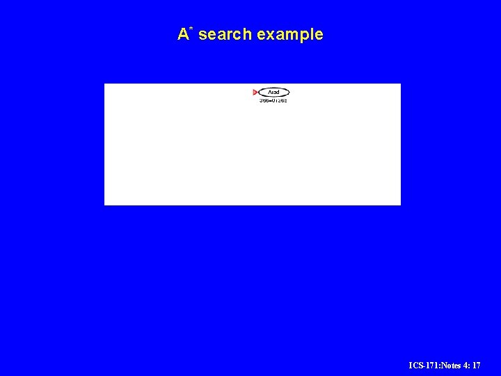
A* search example ICS-171: Notes 4: 17

A* search example ICS-171: Notes 4: 18

A* search example ICS-171: Notes 4: 19

A* search example ICS-171: Notes 4: 20

A* search example ICS-171: Notes 4: 21

A* search example ICS-171: Notes 4: 22

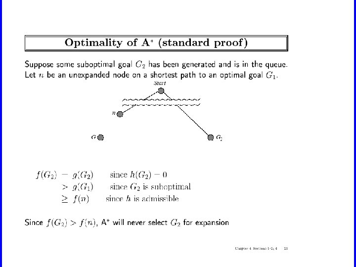
Admissible heuristics ICS-171: Notes 4: 24

ICS-171: Notes 4: 25

ICS-171: Notes 4: 26

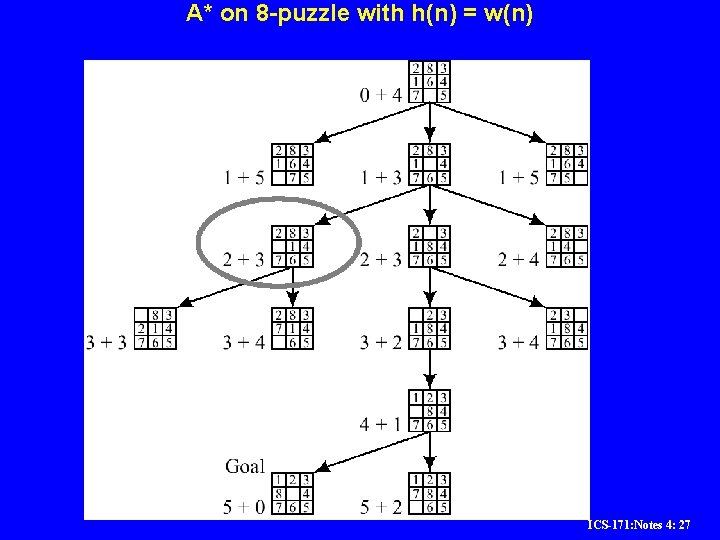
A* on 8 -puzzle with h(n) = w(n) ICS-171: Notes 4: 27

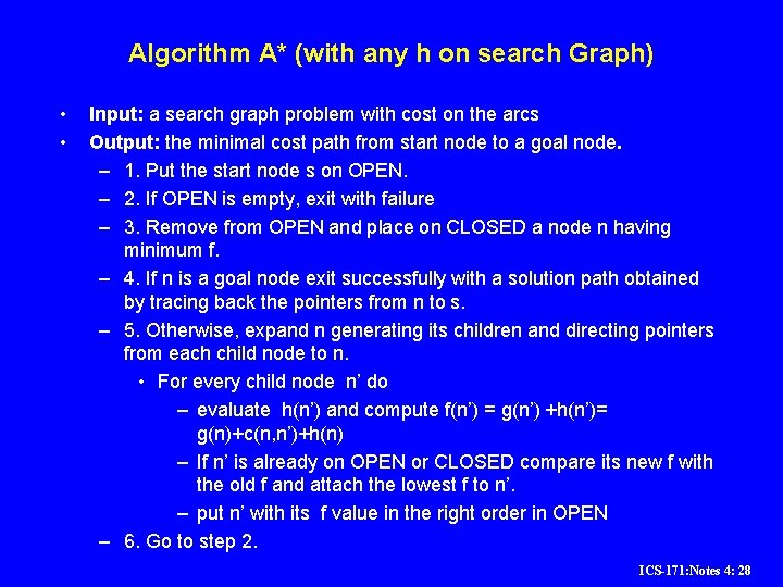
Algorithm A* (with any h on search Graph) • • Input: a search graph problem with cost on the arcs Output: the minimal cost path from start node to a goal node. – 1. Put the start node s on OPEN. – 2. If OPEN is empty, exit with failure – 3. Remove from OPEN and place on CLOSED a node n having minimum f. – 4. If n is a goal node exit successfully with a solution path obtained by tracing back the pointers from n to s. – 5. Otherwise, expand n generating its children and directing pointers from each child node to n. • For every child node n’ do – evaluate h(n’) and compute f(n’) = g(n’) +h(n’)= g(n)+c(n, n’)+h(n) – If n’ is already on OPEN or CLOSED compare its new f with the old f and attach the lowest f to n’. – put n’ with its f value in the right order in OPEN – 6. Go to step 2. ICS-171: Notes 4: 28

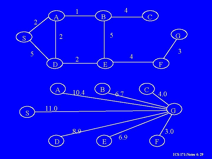
2 1 A 5 D A S B C 5 2 S 4 2 10. 4 G 3 4 F E B 6. 7 C 4. 0 11. 0 G 8. 9 D E 6. 9 3. 0 F ICS-171: Notes 4: 29

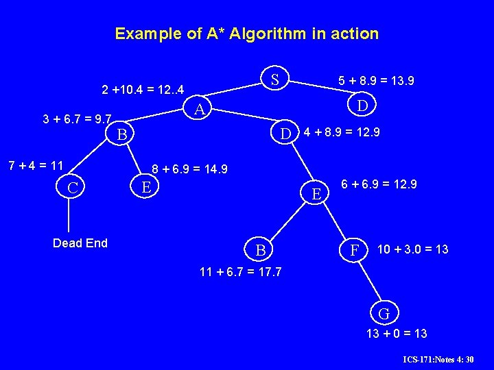
Example of A* Algorithm in action S 2 +10. 4 = 12. . 4 3 + 6. 7 = 9. 7 5 + 8. 9 = 13. 9 D A D B 7 + 4 = 11 4 + 8. 9 = 12. 9 8 + 6. 9 = 14. 9 C Dead End E E B 6 + 6. 9 = 12. 9 F 10 + 3. 0 = 13 11 + 6. 7 = 17. 7 G 13 + 0 = 13 ICS-171: Notes 4: 30

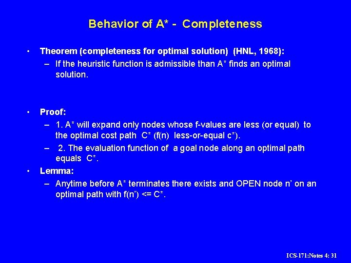
Behavior of A* - Completeness • Theorem (completeness for optimal solution) (HNL, 1968): – If the heuristic function is admissible than A* finds an optimal solution. • Proof: – 1. A* will expand only nodes whose f-values are less (or equal) to the optimal cost path C* (f(n) less-or-equal c*). – 2. The evaluation function of a goal node along an optimal path equals C*. Lemma: – Anytime before A* terminates there exists and OPEN node n’ on an optimal path with f(n’) <= C*. • ICS-171: Notes 4: 31

ICS-171: Notes 4: 32

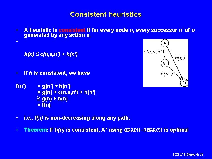
Consistent heuristics • A heuristic is consistent if for every node n, every successor n' of n generated by any action a, • h(n) ≤ c(n, a, n') + h(n') • If h is consistent, we have f(n') = g(n') + h(n') = g(n) + c(n, a, n') + h(n') ≥ g(n) + h(n) = f(n) • i. e. , f(n) is non-decreasing along any path. • Theorem: If h(n) is consistent, A* using GRAPH-SEARCH is optimal ICS-171: Notes 4: 33

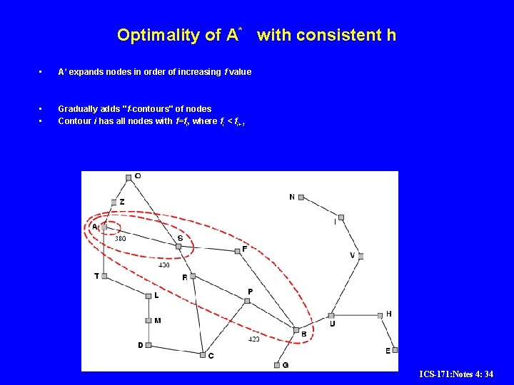
Optimality of A* with consistent h • A* expands nodes in order of increasing f value • • Gradually adds "f-contours" of nodes Contour i has all nodes with f=fi, where fi < fi+1 ICS-171: Notes 4: 34

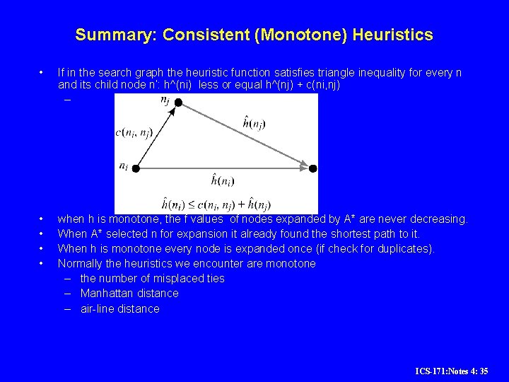
Summary: Consistent (Monotone) Heuristics • If in the search graph the heuristic function satisfies triangle inequality for every n and its child node n’: h^(ni) less or equal h^(nj) + c(ni, nj) – • • when h is monotone, the f values of nodes expanded by A* are never decreasing. When A* selected n for expansion it already found the shortest path to it. When h is monotone every node is expanded once (if check for duplicates). Normally the heuristics we encounter are monotone – the number of misplaced ties – Manhattan distance – air-line distance ICS-171: Notes 4: 35

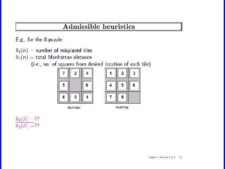
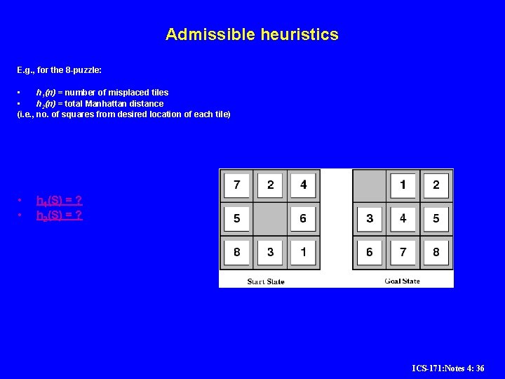
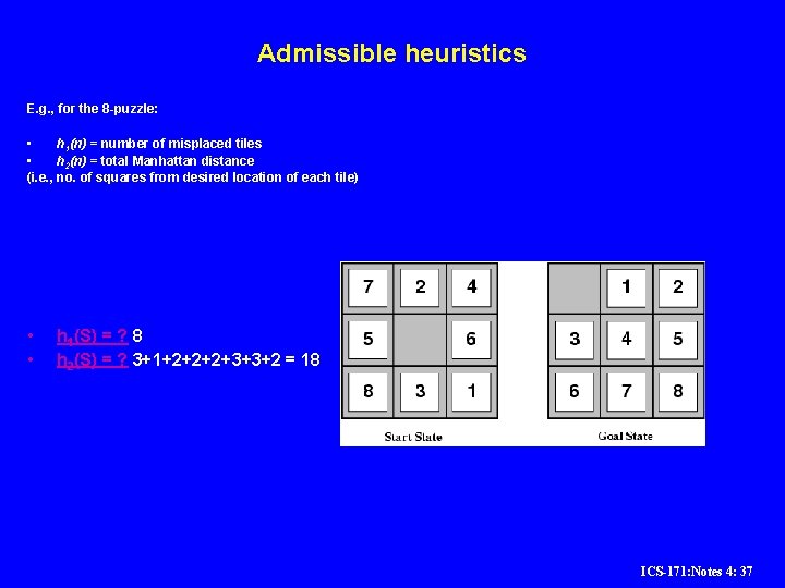
Admissible heuristics E. g. , for the 8 -puzzle: • h 1(n) = number of misplaced tiles • h 2(n) = total Manhattan distance (i. e. , no. of squares from desired location of each tile) • • h 1(S) = ? h 2(S) = ? ICS-171: Notes 4: 36

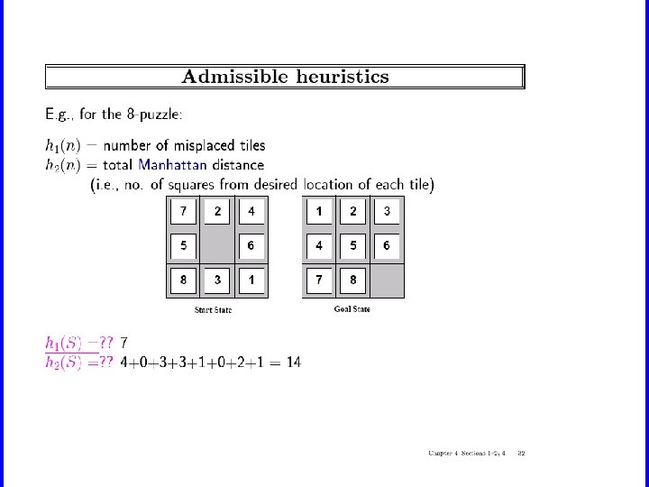
Admissible heuristics E. g. , for the 8 -puzzle: • h 1(n) = number of misplaced tiles • h 2(n) = total Manhattan distance (i. e. , no. of squares from desired location of each tile) • • h 1(S) = ? 8 h 2(S) = ? 3+1+2+2+2+3+3+2 = 18 ICS-171: Notes 4: 37

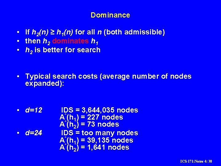
Dominance • If h 2(n) ≥ h 1(n) for all n (both admissible) • then h 2 dominates h 1 • h 2 is better for search • Typical search costs (average number of nodes expanded): • d=12 • d=24 IDS = 3, 644, 035 nodes A*(h 1) = 227 nodes A*(h 2) = 73 nodes IDS = too many nodes A*(h 1) = 39, 135 nodes A*(h 2) = 1, 641 nodes ICS-171: Notes 4: 38

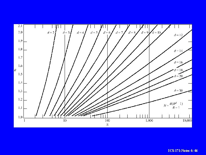
Complexity of A* • • • A* is optimally efficient (Dechter and Pearl 1985): – It can be shown that all algorithms that do not expand a node which A* did expand (inside the contours) may miss an optimal solution A* worst-case time complexity: – is exponential unless the heuristic function is very accurate If h is exact (h = h*) – search focus only on optimal paths Main problem: space complexity is exponential Effective branching factor: – logarithm of base (d+1) of average number of nodes expanded. ICS-171: Notes 4: 39

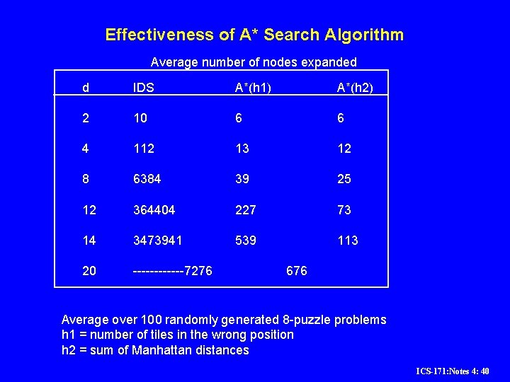
Effectiveness of A* Search Algorithm Average number of nodes expanded d IDS A*(h 1) A*(h 2) 2 10 6 6 4 112 13 12 8 6384 39 25 12 364404 227 73 14 3473941 539 113 20 ------7276 676 Average over 100 randomly generated 8 -puzzle problems h 1 = number of tiles in the wrong position h 2 = sum of Manhattan distances ICS-171: Notes 4: 40

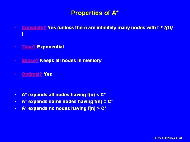
Properties of A* • Complete? Yes (unless there are infinitely many nodes with f ≤ f(G) ) • Time? Exponential • Space? Keeps all nodes in memory • Optimal? Yes • • • A* expands all nodes having f(n) < C* A* expands some nodes having f(n) = C* A* expands no nodes having f(n) > C* ICS-171: Notes 4: 41

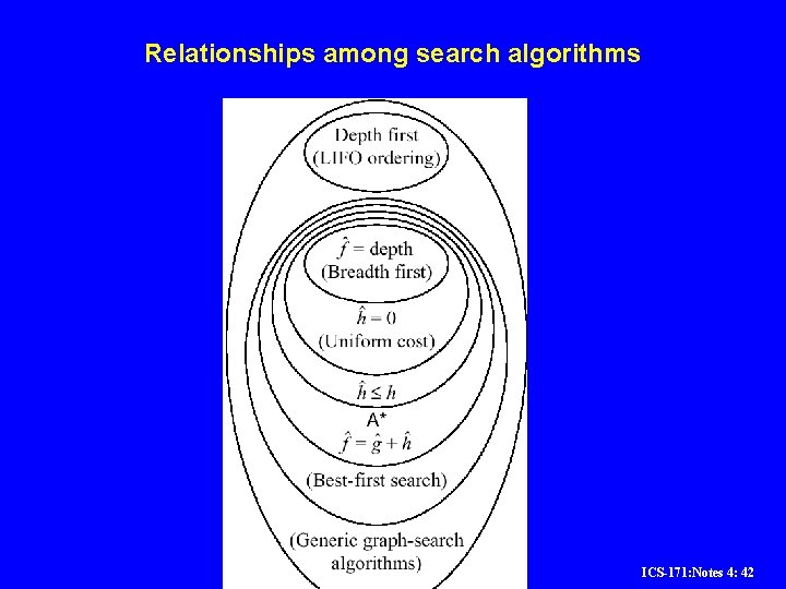
Relationships among search algorithms ICS-171: Notes 4: 42

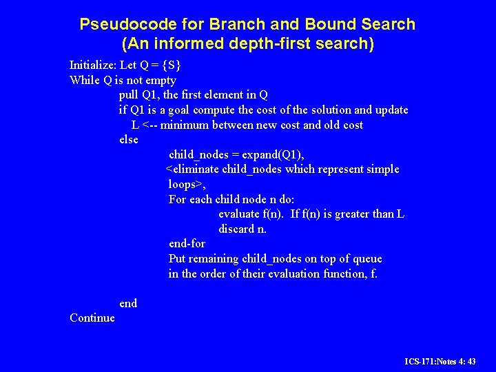
Pseudocode for Branch and Bound Search (An informed depth-first search) Initialize: Let Q = {S} While Q is not empty pull Q 1, the first element in Q if Q 1 is a goal compute the cost of the solution and update L <-- minimum between new cost and old cost else child_nodes = expand(Q 1), <eliminate child_nodes which represent simple loops>, For each child node n do: evaluate f(n). If f(n) is greater than L discard n. end-for Put remaining child_nodes on top of queue in the order of their evaluation function, f. end Continue ICS-171: Notes 4: 43

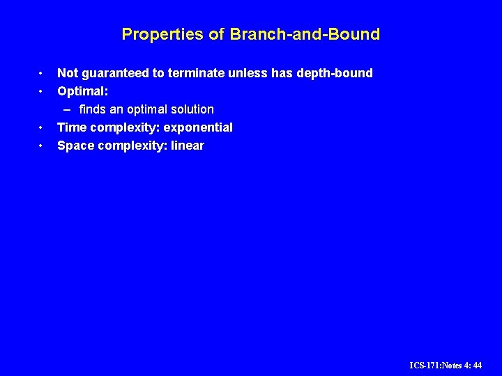
Properties of Branch-and-Bound • • Not guaranteed to terminate unless has depth-bound Optimal: – finds an optimal solution Time complexity: exponential Space complexity: linear ICS-171: Notes 4: 44

Iterative Deepening A* (IDA*) (combining Branch-and-Bound and A*) • • Initialize: f <-- the evaluation function of the start node until goal node is found – Loop: • Do Branch-and-bound with upper-bound L equal current evaluation function • Increment evaluation function to next contour level – end continue Properties: – Guarantee to find an optimal solution – time: exponential, like A* – space: linear, like B&B. ICS-171: Notes 4: 45

ICS-171: Notes 4: 46

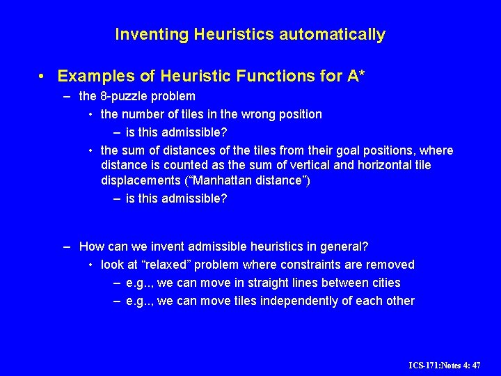
Inventing Heuristics automatically • Examples of Heuristic Functions for A* – the 8 -puzzle problem • the number of tiles in the wrong position – is this admissible? • the sum of distances of the tiles from their goal positions, where distance is counted as the sum of vertical and horizontal tile displacements (“Manhattan distance”) – is this admissible? – How can we invent admissible heuristics in general? • look at “relaxed” problem where constraints are removed – e. g. . , we can move in straight lines between cities – e. g. . , we can move tiles independently of each other ICS-171: Notes 4: 47

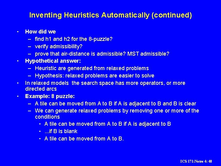
Inventing Heuristics Automatically (continued) • • How did we – find h 1 and h 2 for the 8 -puzzle? – verify admissibility? – prove that air-distance is admissible? MST admissible? Hypothetical answer: – Heuristic are generated from relaxed problems – Hypothesis: relaxed problems are easier to solve In relaxed models the search space has more operators, or more directed arcs Example: 8 puzzle: – A tile can be moved from A to B if A is adjacent to B and B is clear – We can generate relaxed problems by removing one or more of the conditions • A tile can be moved from A to B if A is adjacent to B • . . . if B is blank • A tile can be moved from A to B. ICS-171: Notes 4: 48

Relaxed problems • A problem with fewer restrictions on the actions is called a relaxed problem • The cost of an optimal solution to a relaxed problem is an admissible heuristic for the original problem • If the rules of the 8 -puzzle are relaxed so that a tile can move anywhere, then h 1(n) gives the shortest solution • If the rules are relaxed so that a tile can move to any adjacent square, then h 2(n) gives the shortest ICS-171: Notes 4: 50 solution

ICS-171: Notes 4: 51

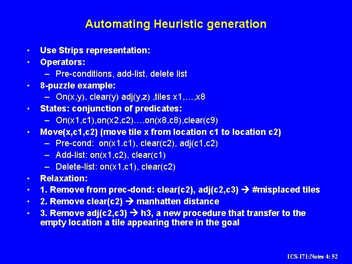
Automating Heuristic generation • • • Use Strips representation: Operators: – Pre-conditions, add-list, delete list 8 -puzzle example: – On(x, y), clear(y) adj(y, z) , tiles x 1, …, x 8 States: conjunction of predicates: – On(x 1, c 1), on(x 2, c 2)…. on(x 8, c 8), clear(c 9) Move(x, c 1, c 2) (move tile x from location c 1 to location c 2) – Pre-cond: on(x 1. c 1), clear(c 2), adj(c 1, c 2) – Add-list: on(x 1, c 2), clear(c 1) – Delete-list: on(x 1, c 1), clear(c 2) Relaxation: 1. Remove from prec-dond: clear(c 2), adj(c 2, c 3) #misplaced tiles 2. Remove clear(c 2) manhatten distance 3. Remove adj(c 2, c 3) h 3, a new procedure that transfer to the empty location a tile appearing there in the goal ICS-171: Notes 4: 52

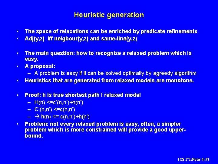
Heuristic generation • • The space of relaxations can be enriched by predicate refinements Adj(y, z) iff neigbour(y, z) and same-line(y, z) • The main question: how to recognize a relaxed problem which is easy. A proposal: – A problem is easy if it can be solved optimally by agreedy algorithm Heuristics that are generated from relaxed models are monotone. • • Proof: h is true shortest path I relaxed model – H(n) <=c’(n, n’)+h(n’) – C’(n, n’) <=c(n, n’) – h(n) <= c(n, n’)+h(n’) Problem: not every relaxed problem is easy, often, a simpler problem which is more constrained will provide a good upperbound. ICS-171: Notes 4: 53

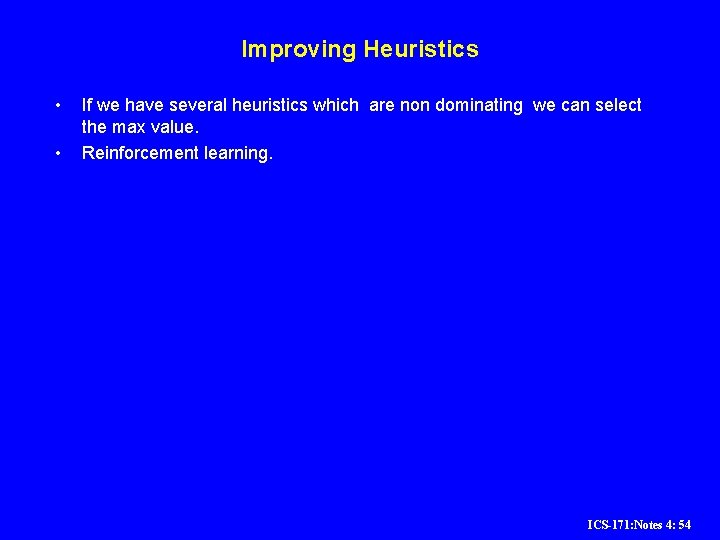
Improving Heuristics • • If we have several heuristics which are non dominating we can select the max value. Reinforcement learning. ICS-171: Notes 4: 54

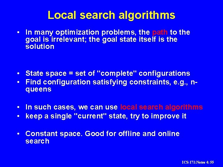
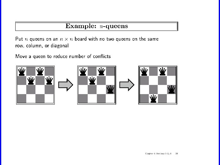
Local search algorithms • In many optimization problems, the path to the goal is irrelevant; the goal state itself is the solution • State space = set of "complete" configurations • Find configuration satisfying constraints, e. g. , nqueens • In such cases, we can use local search algorithms • keep a single "current" state, try to improve it • Constant space. Good for offline and online search ICS-171: Notes 4: 55

ICS-171: Notes 4: 56

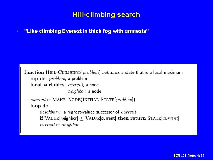
Hill-climbing search • "Like climbing Everest in thick fog with amnesia" ICS-171: Notes 4: 57

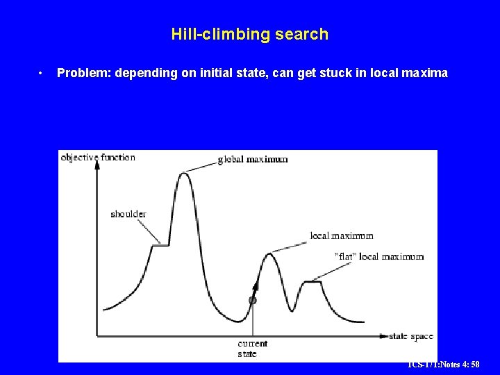
Hill-climbing search • Problem: depending on initial state, can get stuck in local maxima ICS-171: Notes 4: 58

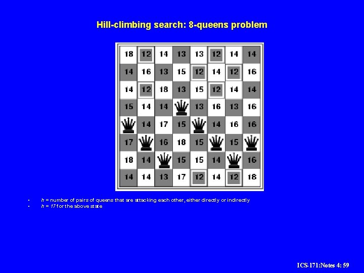
Hill-climbing search: 8 -queens problem • • h = number of pairs of queens that are attacking each other, either directly or indirectly h = 17 for the above state ICS-171: Notes 4: 59

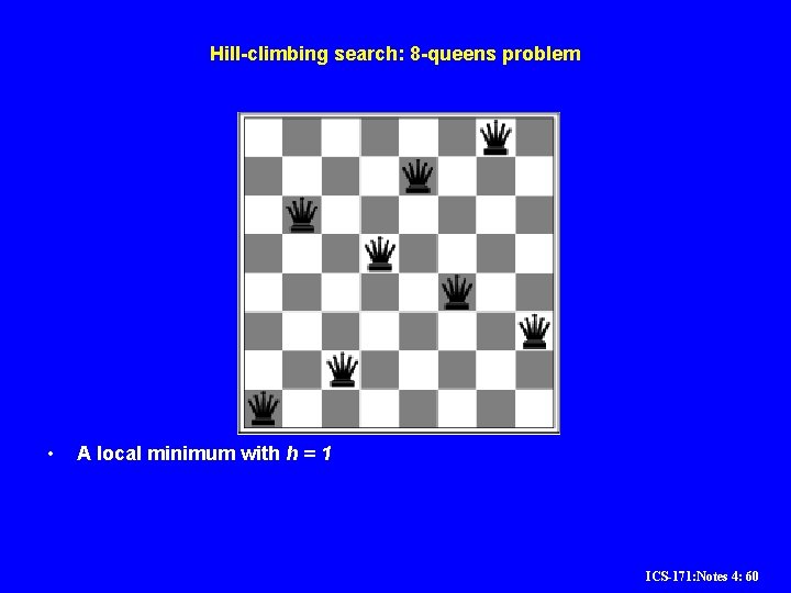
Hill-climbing search: 8 -queens problem • A local minimum with h = 1 ICS-171: Notes 4: 60

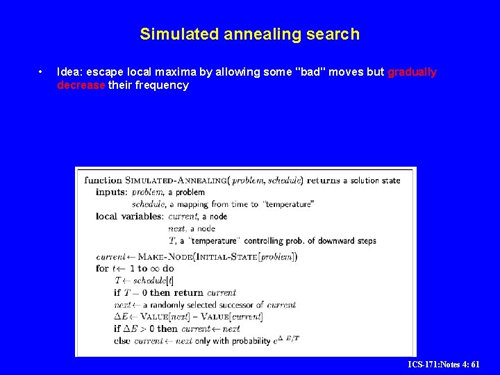
Simulated annealing search • Idea: escape local maxima by allowing some "bad" moves but gradually decrease their frequency ICS-171: Notes 4: 61

Properties of simulated annealing search • One can prove: If T decreases slowly enough, then simulated annealing search will find a global optimum with probability approaching 1 • Widely used in VLSI layout, airline scheduling, etc ICS-171: Notes 4: 62