Inference in Gaussian and Hybrid Bayesian Networks ICS

Inference in Gaussian and Hybrid Bayesian Networks ICS 275 B

Gaussian Distribution

0. 4 gaussian(x, 0, 1) gaussian(x, 1, 1) 0. 35 0. 3 0. 25 0. 2 0. 15 0. 1 0. 05 0 -3 -2 -1 0 N(m, s) 1 2 3

0. 4 gaussian(x, 0, 1) gaussian(x, 0, 2) 0. 35 0. 3 0. 25 0. 2 0. 15 0. 1 0. 05 0 -3 -2 -1 0 1 2 N(m, s) 3

Multivariate Gaussian Definition: Let X 1, …, Xn. Be a set of random variables. A multivariate Gaussian distribution over X 1, …, Xn is a parameterized by an n-dimensional mean vector and an n x n positive definitive covariance matrix . It defines a joint density via:

Multivariate Gaussian

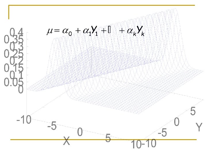
Linear Gaussian Distribution Definition: Let Y be a continuous node with continuous parents X 1, …, Xk. We say that Y has a linear Gaussian model if it can be described using parameters 0, …, k and 2 such that: P(y| x 1, …, xk)=N (μy + 1 x 1 +…, kxk ; ) =N([μy, 1, …, k] , )

A B A B

Linear Gaussian Network Definition Linear Gaussian Bayesian network is a Bayesian network all of whose variables are continuous and where all of the CPTs are linear Gaussians. Linear Gaussian BN Multivariate Gaussian =>Linear Gaussian BN has a compact representation

Inference in Continuous Networks A B

Marginalization

Problems: When we Multiply two arbitrary Gaussians! Inverse of K and M is always well defined. However, this inverse is not!

Theoretical explanation: Why this is the case ? n n n Inverse of a matrix of size n x n exists when the matrix is of rank n. If all sigmas and w’s are assumed to be 1. (K-1+M-1) has rank 2 and so is not invertible.

Density vs conditional n However, q Theorem: If the product of the gaussians represents a multi-variate gaussian density, then the inverse always exists. n n For example, For P(A|B)*P(B)=P(A, B) = N(c, C) then inverse of C always exists. P(A, B) is a multi-variate gaussian (density). But P(A|B)*P(B|X)=P(A, B|X) = N(c, C) then inverse of C may not exist. P(A, B|X) is a conditional gaussian.

Inference: A general algorithm Computing marginal of a given variable, say Z. Step 1: Convert all conditional gaussians to canonical form

Inference: A general algorithm Computing marginal of a given variable, say Z. n Step 2: q Extend all g’s, h’s and k’s to the same domain by adding 0’s.

Inference: A general algorithm Computing marginal of a given variable, say Z. 3: Add all g’s, all h’s and all k’s. n Step 4: Let the variables involved in the computation be: P(X 1, X 2, …, Xk, Z)= N(μ, ∑)

Inference: A general algorithm Computing marginal of a given variable, say Z. Step 5: Extract the marginal

Inference: Computing marginal of a given variable n For a continuous Gaussian Bayesian Network, inference is polynomial O(N 3). q n n Complexity of matrix inversion So algorithms like belief propagation are not generally used when all variables are Gaussian. Can we do better than N^3? q Use Bucket elimination.

Bucket elimination Algorithm elim-bel (Dechter 1996) Marginalization operator bucket B: bucket C: Multiplication operator P(b|a) P(d|b, a) P(e|b, c) P(c|a) B C bucket D: D bucket E: e=0 bucket A: P(a) P(a|e=0) W*=4 ”induced width” (max clique size) E A

Multiplication Operator n n n Convert all functions to canonical form if necessary. Extend all functions to the same variables (g 1, h 1, k 1)*(g 2, h 2, k 2) =(g 1+g 2, h 1+h 2, k 1+k 2)

Again our problem! h(a, d, c, e) does not represent a density and so cannot be computed in our usual form N(μ, σ) Marginalization operator bucket B: bucket C: Multiplication operator P(b|a) P(d|b, a) P(e|b, c) P(c|a) B C bucket D: D bucket E: P(e) bucket A: P(a) W*=4 ”induced width” (max clique size) E A

Solution: Marginalize in canonical form n Although intermediate functions computed in bucket elimination are conditional, we can marginalize in canonical form, so we can eliminate the problem of non-existence of inverse completely.

Algorithm n n n In each bucket, convert all functions in canonical form if necessary, multiply them and marginalize out the variable in the bucket as shown in the previous slide. Theorem: P(A) is a density and is correct. Complexity: Time and space: O((w+1)^3) where w is the width of the ordering used.

Continuous Node, Discrete Parents Definition: Let X be a continuous node, and let U={U 1, U 2, …, Un} be its discrete parents and Y={Y 1, Y 2, …, Yk} be its continuous parents. We say that X has a conditional linear Gaussian (CLG) CPT if, for every value u D(U), we have a a set of (k+1) coefficients au, 0, au, 1, …, au, k+1 and a variance u 2 such that:

CLG Network Definition: A Bayesian network is called a CLG network if every discrete node has only discrete parents, and every continuous node has a CLG CPT.

Inference in CLGs n Can we use the same algorithm? q n Yes, but the algorithm is unbounded if we are not careful. Reason: q Marginalizing out discrete variables from any arbitrary function in CLGs is not bounded. n If we marginalize out y and k from f(x, y, i, k) , the result is a mixture of 4 gaussians instead of 2. q q X and y are continuous variables I and k are discrete binary variables.

Solution: Approximate the mixture of Gaussians by a single gaussian

Multiplication and Strong Marginalization marginal when marginalizing Multiplication n Convert all functions to canonical form if necessary. Extend all functions to the same variables (g 1, h 1, k 1)*(g 2, h 2, k 2) =(g 1+g 2, h 1+h 2, k 1+k 2) continuous variables Weak marginal when marginalizing discrete variables

Problem while using this marginalization in bucket elimination n n Requires computing ∑ and μ which is not possible due to non-existence of inverse. Solution: Use an ordering such that you never have to marginalize out discrete variables from a function that has both discrete and continuous gaussian variables. Special case: Compute marginal at a discrete node Homework: Derive a bucket elimination algorithm for computing marginal of a continuous variable.

Special Case: A marginal on a discrete variable in a CLG is to be computed. B, C and D are continuous variables and A and E is discrete Marginalization operator Multiplication operator bucket B: P(b|a, e) P(d|b, a) P(d|b, c) bucket C: P(c|a) bucket D: bucket E: P(e) bucket A: P(a) W*=4 ”induced width” (max clique size)

Complexity of the special case n n Discrete-width (wd): Maximum number of discrete variables in a clique Continuous-width (wc): Maximum number of continuous variables in a clique Time: O(exp(wd)+wc^3) Space: O(exp(wd)+wc^3)

Algorithm for the general case: Computing Belief at a continuous node of a CLG n Convert all functions to canonical form. n n Create a special tree-decomposition Assign functions to appropriate cliques (Same as assigning functions to buckets) Select a Strong Root Perform message passing

Creating a Special-tree decomposition n n Moralize the Bayesian Network. Select an ordering such that all continuous variables are ordered before discrete variables (Increases induced width).

Elimination order w x y z Strong elimination order: • First eliminate continuous variables • Eliminate discrete variable when no available continuous variables W and X are discrete variables and Y and Z are continuous. Moralized graph has this edge

Elimination order (1) dim: 2 w x y dim: 2 z 1

Elimination order (2) dim: 2 w x y 2 z 1

Elimination order (3) 3 dim: 2 w x y 2 z 1

Elimination order (4) 3 4 w 3 x w x 3 y w 2 y 2 3 z 4 Cliques 2 w y 1 2 y 2 z Cliques 1 1 separator

Bucket tree or Junction tree (1) w w x y Cliques 2: root w y separator y z Cliques 1

Algorithm for the general case: Computing Belief at a continuous node of a CLG n n n Convert all functions to canonical form. Create a special tree-decomposition Assign functions to appropriate cliques (Same as assigning functions to buckets) Select a Strong Root Perform message passing

Assigning Functions to cliques n Select a function and place it in an arbitrary clique that mentions all variables in the function.

Algorithm for the general case: Computing Belief at a continuous node of a CLG n n n Convert all functions to canonical form. Create a special tree-decomposition Assign functions to appropriate cliques (Same as assigning functions to buckets) Select a Strong Root Perform message passing

Strong Root n We define a strong root as any node R in the buckettree which satisfies the following property: for any pair (V, W) which are neighbors on the tree with W closer to R than V, we have

Example Strong root Strong Root

Algorithm for the general case: Computing Belief at a continuous node of a CLG n n Create a special tree-decomposition Assign functions to appropriate cliques (Same as assigning functions to buckets) Select a Strong Root Perform message passing

Message passing atx 2 a typical node x 1 a b o. Node “a” contains functions assigned to it according to the tree-decomposition scheme denoted by pj(a)

Message Passing Two pass algorithm: Bucket-tree propagation Distribute Collect root Figure from P. Green

Lets look at the messages Collect Evidence Strong Root ∫C ∫D ∫L ∫Min∫D ∫Mout

Distribute Evidence Strong Root ∫E∑W, B ∑F ∫E∑W, B ∫E∑B ∑W

Lauritzens theorem n When you perform message passing such that collect evidence contains only strong marginals and distribute evidence may contain weak marginals, the junction-tree algorithm in exact in the sense that: q The first (mean) and second moments (variance) computed are true moments

Complexity n n n Polynomial in #of continuous variables in a clique (n 3) Exponential in #of discrete variables in a clique Possible options for approximation q q Ignore the strong root assumption and use approximation like MBTE, IJGP, Sampling Respect the strong root assumption and use approximation like MBTE, IJGP, Sampling n Inaccuracies only due to discrete variables if done in one pass of MBTE.

Initialization (1) dim: 2 w= 0 0. 5 w= 1 0. 5 dim: 2 w x x=0 0. 4 x=1 0. 6 X=0 y dim: 2 z W=0 dim: 2 W=1 X=1

Initialization (2) Cliques 1 wyz Cliques 2 (root) wy wxy x=0 w=0 g=log(0. 5), h=[], K=[ ] w=1 g=log(0. 5), h=[], K=[ ] W=0 g = -4. 0629 h = [0. 0889 -0. 0111 -0. 0556] K= x=1 g=log(0. 4), h=[], K=[ ] g=log(0. 6), h=[], K=[ ] X=0 g = -4. 1245 h = [-0. 02 0. 12]’ K = [0. 1 0; 0 0. 1] W=1 g = -2. 7854 h = [0. 0867 -0. 0633 -0. 1000 -0. 1667] K= X=1 g = -3. 0310 h = [0. 5 -0. 5]’ K = [0. 5; 0. 5]

Initialization (3) Cliques 1 wyz Cliques 2 (root) wxy wy empty wx=00 wx=10 g = -5. 1308 h = [-0. 02 0. 12]’ K = [0. 1 0; 0 0. 1] wx=01 g = -3. 5418 h = [0. 5 -0. 5]’ K = [0. 5; 0. 5] W=0 g = -4. 7560 h= K= W=1 g = -3. 4786 h= K= wx=11 g = -3. 5418 h = [0. 5 -0. 5]’ K = [0. 5; 0. 5]

Message Passing Cliques 1 wyz Collect evidence Cliques 2 (root) wy empty wxy Distribute evidence

Collect evidence (1) Cliques 1 wyz Cliques 2 (root) wy empty wxy y 2 y 3 y 2 (y 1, y 2) (y 2) y 1 y 2

Collect evidence (2) Cliques 1 wyz Cliques 2 (root) wxy wy empty W=0 g = -4. 7560 h= K= W=1 g = -3. 4786 h= K= marginalization W=0 g = -0. 6931 h = [0. 1388 0]’ *1. 0 e-16 K = [0. 2776 -0. 0694; 0. 0347 0]*1. 0 e-16 W=1 g = -0. 6931 h = [0 0]’ K = [0 0 0 0]

Collect evidence (3) Cliques 1 Cliques 2 (root) wyz wxy wy empty W=0 W=1 g = -0. 6931 h = [0. 1388 0]’ *1. 0 e-16 K = [0. 2776 -0. 0694; 0. 0347 0]*1. 0 e-16 g = -0. 6931 h = [0 0]’ K = [0 0 0 0] multiplication wx=00 wx=10 g = -5. 1308 h = [-0. 02 0. 12]’ K = [0. 1 0; 0 0. 1] wx=00 wx=10 g = -5. 8329 h = [-0. 02 0. 12]’ K = [0. 1 0; 0 0. 1] wx=01 g = -3. 5418 h = [0. 5 -0. 5]’ K = [0. 5; 0. 5] wx=01 g = -4. 2350 h = [0. 5 -0. 5]’ K = [0. 5; 0. 5] wx=11 g = -3. 5418 h = [0. 5 -0. 5]’ K = [0. 5; 0. 5] wx=11 g = -4. 2350 h = [0. 5 -0. 5]’ K = [0. 5; 0. 5]

Distribute evidence (1) Cliques 1 wyz Cliques 2 (root) wxy wy W=0 g = -4. 7560 h= K= W=1 g = -3. 4786 h= K= division W=0 g = -0. 6931 h = [0. 1388 0]’ *1. 0 e-16 K = [0. 2776 -0. 0694; 0. 0347 0]*1. 0 e-16 W=1 g = -0. 6931 h = [0 0]’ K = [0 0 0 0]

Distribute evidence (2) Cliques 1 wyz Cliques 2 (root) wy wxy W=0 g = -4. 0629 h= K= W=1 g = -2. 7854 h= K=

Distribute evidence (3) Cliques 1 Cliques 2 (root) wyz wxy wy wx=00 wx=10 g = -5. 8329 h = [-0. 02 0. 12]’ K = [0. 1 0; 0 0. 1] wx=01 g = -4. 2350 h = [0. 5 -0. 5]’ K = [0. 5; 0. 5] Marginalize over x w=0 logp = -0. 6931 mu = [0. 52 -0. 12]’ Sigma = w=1 logp = -0. 6931 mu = [0. 52 -0. 12]’ Sigma = wx=11 g = -4. 2350 h = [0. 5 -0. 5]’ K = [0. 5; 0. 5]

Distribute evidence (4) Cliques 1 Cliques 2 (root) wyz wxy wy W=0 W=1 g = -4. 0629 h= K= g = -2. 7854 h= K= multiplication w=0 logp = -0. 6931 mu = [0. 52 -0. 12]’ Sigma = w=1 logp = -0. 6931 mu = [0. 52 -0. 12]’ Sigma = w=0 g = -4. 3316 h = [0. 0927 -0. 0096]’ K= w=1 g = -0. 6931 h = [0. 0927 -0. 0096]’ K= Canonical form