Inference in First Order Logic Some material adopted

Inference in First Order Logic Some material adopted from notes by Tim Finin, Andreas Geyer-Schulz, and Chuck Dyer 1

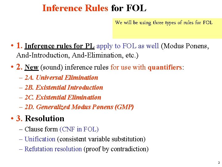
Inference Rules for FOL We will be using three types of rules for FOL • 1. Inference rules for PL apply to FOL as well (Modus Ponens, And-Introduction, And-Elimination, etc. ) • 2. New (sound) inference rules for use with quantifiers: – 2 A. Universal Elimination – 2 B. Existential Introduction – 2 C. Existential Elimination – 2 D. Generalized Modus Ponens (GMP) • 3. Resolution – Clause form (CNF in FOL) – Unification (consistent variable substitution) – Refutation resolution (proof by contradiction) 2

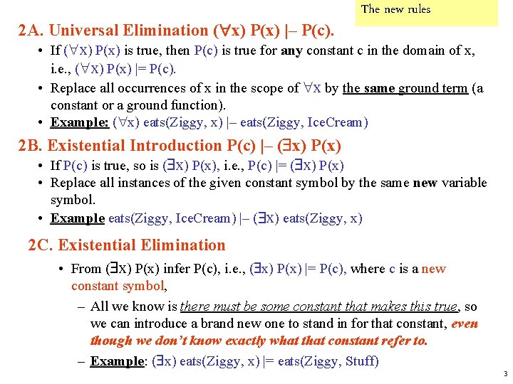
2 A. Universal Elimination ( x) P(x) |– P(c). The new rules • If ( x) P(x) is true, then P(c) is true for any constant c in the domain of x, i. e. , ( x) P(x) |= P(c). • Replace all occurrences of x in the scope of x by the same ground term (a constant or a ground function). • Example: ( x) eats(Ziggy, x) |– eats(Ziggy, Ice. Cream) 2 B. Existential Introduction P(c) |– ( x) P(x) • If P(c) is true, so is ( x) P(x), i. e. , P(c) |= ( x) P(x) • Replace all instances of the given constant symbol by the same new variable symbol. • Example eats(Ziggy, Ice. Cream) |– ( x) eats(Ziggy, x) 2 C. Existential Elimination • From ( x) P(x) infer P(c), i. e. , ( x) P(x) |= P(c), where c is a new constant symbol, – All we know is there must be some constant that makes this true, so we can introduce a brand new one to stand in for that constant, even though we don’t know exactly what that constant refer to. – Example: ( x) eats(Ziggy, x) |= eats(Ziggy, Stuff) 3

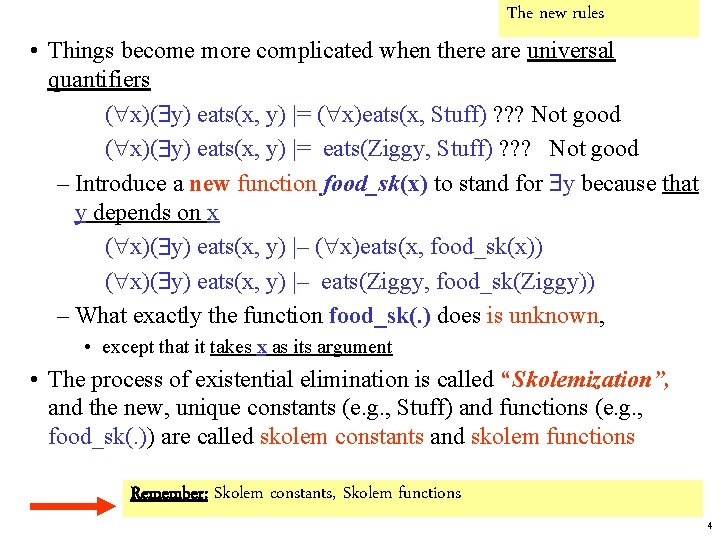
The new rules • Things become more complicated when there are universal quantifiers ( x)( y) eats(x, y) |= ( x)eats(x, Stuff) ? ? ? Not good ( x)( y) eats(x, y) |= eats(Ziggy, Stuff) ? ? ? Not good – Introduce a new function food_sk(x) to stand for y because that y depends on x ( x)( y) eats(x, y) |– ( x)eats(x, food_sk(x)) ( x)( y) eats(x, y) |– eats(Ziggy, food_sk(Ziggy)) – What exactly the function food_sk(. ) does is unknown, • except that it takes x as its argument • The process of existential elimination is called “Skolemization”, and the new, unique constants (e. g. , Stuff) and functions (e. g. , food_sk(. )) are called skolem constants and skolem functions Remember: Skolem constants, Skolem functions 4

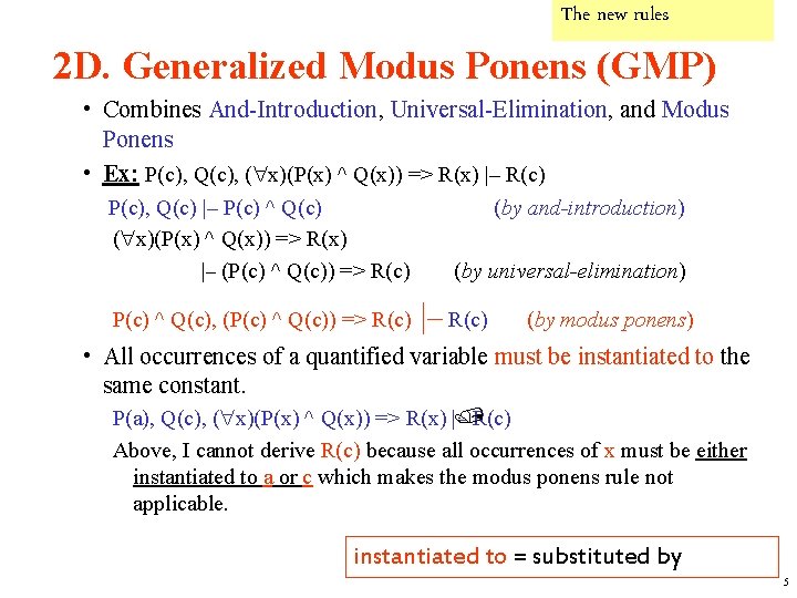
The new rules 2 D. Generalized Modus Ponens (GMP) • Combines And-Introduction, Universal-Elimination, and Modus Ponens • Ex: P(c), Q(c), ( x)(P(x) ^ Q(x)) => R(x) |– R(c) P(c), Q(c) |– P(c) ^ Q(c) ( x)(P(x) ^ Q(x)) => R(x) |– (P(c) ^ Q(c)) => R(c) P(c) ^ Q(c), (P(c) ^ Q(c)) => R(c) (by and-introduction) (by universal-elimination) |– R(c) (by modus ponens) • All occurrences of a quantified variable must be instantiated to the same constant. P(a), Q(c), ( x)(P(x) ^ Q(x)) => R(x) | – R(c) Above, I cannot derive R(c) because all occurrences of x must be either instantiated to a or c which makes the modus ponens rule not applicable. instantiated to = substituted by 5

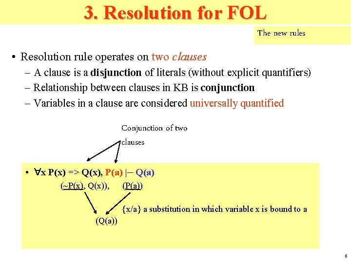
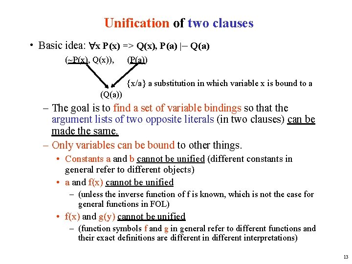
3. Resolution for FOL The new rules • Resolution rule operates on two clauses – A clause is a disjunction of literals (without explicit quantifiers) – Relationship between clauses in KB is conjunction – Variables in a clause are considered universally quantified Conjunction of two clauses • x P(x) => Q(x), P(a) |– Q(a) (~P(x), Q(x)), (P(a)) {x/a} a substitution in which variable x is bound to a (Q(a)) 6

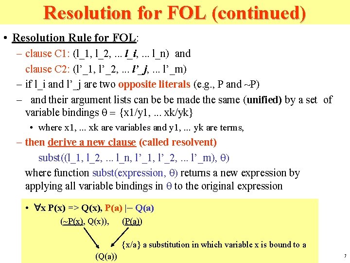
Resolution for FOL (continued) • Resolution Rule for FOL: – clause C 1: (l_1, l_2, . . . l_i, . . . l_n) and clause C 2: (l’_1, l’_2, . . . l’_j, . . . l’_m) – if l_i and l’_j are two opposite literals (e. g. , P and ~P) – and their argument lists can be be made the same (unified) by a set of variable bindings q = {x 1/y 1, . . . xk/yk} • where x 1, . . . xk are variables and y 1, . . . yk are terms, – then derive a new clause (called resolvent) subst((l_1, l_2, . . . l_n, l’_1, l’_2, . . . l’_m), q) where function subst(expression, q) returns a new expression by applying all variable bindings in q to the original expression • x P(x) => Q(x), P(a) |– Q(a) (~P(x), Q(x)), (P(a)) {x/a} a substitution in which variable x is bound to a (Q(a)) 7

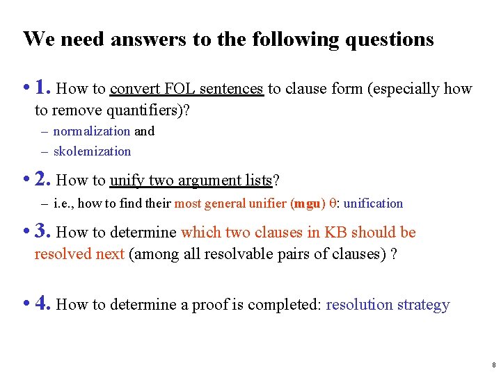
We need answers to the following questions • 1. How to convert FOL sentences to clause form (especially how to remove quantifiers)? – normalization and – skolemization • 2. How to unify two argument lists? – i. e. , how to find their most general unifier (mgu) q: unification • 3. How to determine which two clauses in KB should be resolved next (among all resolvable pairs of clauses) ? • 4. How to determine a proof is completed: resolution strategy 8

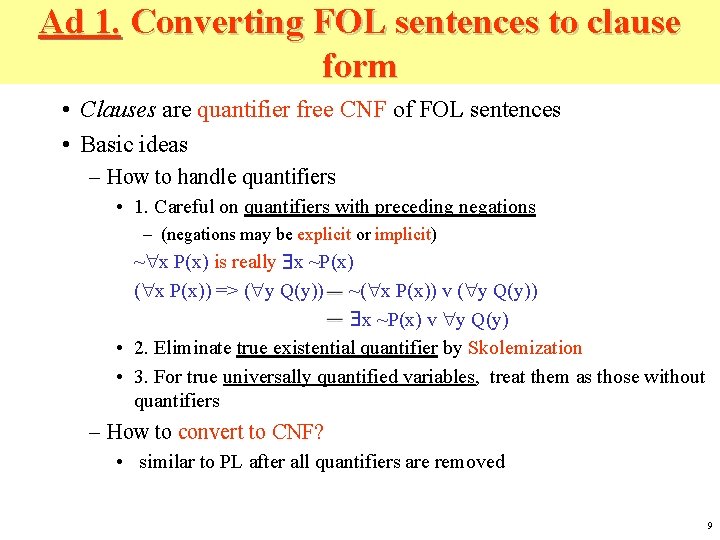
Ad 1. Converting FOL sentences to clause form • Clauses are quantifier free CNF of FOL sentences • Basic ideas – How to handle quantifiers • 1. Careful on quantifiers with preceding negations – (negations may be explicit or implicit) ~ x P(x) is really x ~P(x) ( x P(x)) => ( y Q(y)) ~( x P(x)) v ( y Q(y)) x ~P(x) v y Q(y) • 2. Eliminate true existential quantifier by Skolemization • 3. For true universally quantified variables, treat them as those without quantifiers – How to convert to CNF? • similar to PL after all quantifiers are removed 9

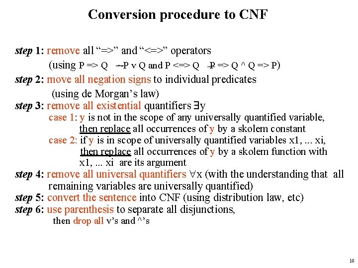
Conversion procedure to CNF step 1: remove all “=>” and “<=>” operators (using P => Q ~P v Q and P <=> Q P => Q ^ Q => P) step 2: move all negation signs to individual predicates (using de Morgan’s law) step 3: remove all existential quantifiers y case 1: y is not in the scope of any universally quantified variable, then replace all occurrences of y by a skolem constant case 2: if y is in scope of universally quantified variables x 1, . . . xi, then replace all occurrences of y by a skolem function with x 1, . . . xi are its argument step 4: remove all universal quantifiers x (with the understanding that all remaining variables are universally quantified) step 5: convert the sentence into CNF (using distribution law, etc) step 6: use parenthesis to separate all disjunctions, then drop all v’s and ^’s 10

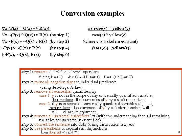
Conversion examples x (P(x) ^ Q(x) => R(x)) x ~(P(x) ^ Q(x)) v R(x) (by step 1) x ~P(x) v ~Q(x) v R(x) (by step 2) ~P(x) v ~Q(x) v R(x) (by step 4) (~P(x), ~Q(x), R(x)) (by step 6) y rose(y) ^ yellow(y) rose(c) ^ yellow(c) (where c is a skolem constant) (rose(c)), (yellow(c)) step 1: remove all “=>” and “<=>” operators (using P => Q ~P v Q and P <=> Q P => Q ^ Q => P) step 2: move all negation signs to individual predicates (using de Morgan’s law) step 3: remove all existential quantifiers y case 1: y is not in the scope of any universally quantified variable, then replace all occurrences of y by a skolem constant case 2: if y is in scope of universally quantified variables x 1, . . . xi, then replace all occurrences of y by a skolem function with x 1, . . . xi are its argument step 4: remove all universal quantifiers x (with the understanding that all remaining variables are universally quantified) step 5: convert the sentence into CNF (using distribution law, etc) step 6: use parenthesis to separate all disjunctions, then drop all v’s and ^’s 11

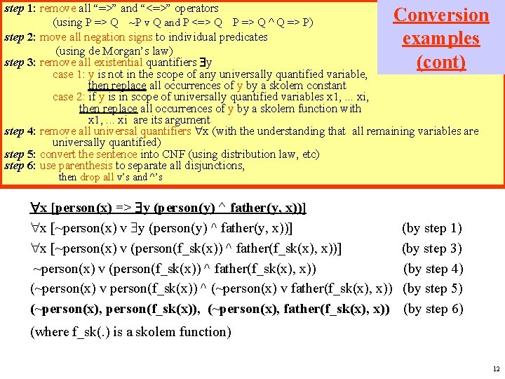
step 1: remove all “=>” and “<=>” operators (using P => Q ~P v Q and P <=> Q P => Q ^ Q => P) step 2: move all negation signs to individual predicates (using de Morgan’s law) step 3: remove all existential quantifiers y case 1: y is not in the scope of any universally quantified variable, replace all occurrences of y by a skolem x (P(x) ^then Q(x) => R(x)) yconstant rose(y) ^ yellow(y) case 2: if y is in scope of universally quantified variables x 1, . . . xi, x ~(P(x) ^ Q(x)) R(x) (by step rose(c) ^ yellow(c) then replacevall occurrences of 1) y by a skolem function with x 1, . . . xi are its argument x ~P(x) v ~Q(x) vquantifiers R(x) (by x step 2) the understanding (where a skolemvariables constant) step 4: remove all universal (with that callisremaining are universally quantified) ~P(x) v ~Q(x) v R(x) (by step 4) (rose(c)), (yellow(c)) step 5: convert the sentence into CNF (using distribution law, etc) step 6: use parenthesis separate all(by disjunctions, (~P(x), ~Q(x), to. R(x)) step 6) Conversion examples (cont) then drop all v’s and ^’s x [person(x) => y (person(y) ^ father(y, x))] x [~person(x) v (person(f_sk(x)) ^ father(f_sk(x), x))] ~person(x) v (person(f_sk(x)) ^ father(f_sk(x), x)) (~person(x) v person(f_sk(x)) ^ (~person(x) v father(f_sk(x), x)) (~person(x), person(f_sk(x)), (~person(x), father(f_sk(x), x)) (by step 1) (by step 3) (by step 4) (by step 5) (by step 6) (where f_sk(. ) is a skolem function) 12

Unification of two clauses • Basic idea: x P(x) => Q(x), P(a) |– Q(a) (~P(x), Q(x)), (P(a)) {x/a} a substitution in which variable x is bound to a (Q(a)) – The goal is to find a set of variable bindings so that the argument lists of two opposite literals (in two clauses) can be made the same. – Only variables can be bound to other things. • Constants a and b cannot be unified (different constants in general refer to different objects) • a and f(x) cannot be unified – (unless the inverse function of f is known, which is not the case for general functions in FOL) • f(x) and g(y) cannot be unified – (function symbols f and g in general refer to different functions and their exact definitions are different interpretations) 13

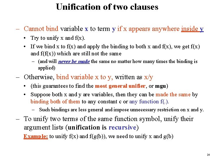
Unification of two clauses – Cannot bind variable x to term y if x appears anywhere inside y • Try to unify x and f(x). • If we bind x to f(x) and apply the binding to both x and f(x), we get f(x) and f(f(x)) which are still not the same – (and will never be made the same no matter how many times the binding is applied) – Otherwise, bind variable x to y, written as x/y • (this guarantees to find the most general unifier, or mgu) • Suppose both x and y are variables, then they can be made the same by binding both of them to any constant c or any function f(. ). – Such bindings are less general and impose unnecessary restriction on x and y. – To unify two terms of the same function symbol, unify their argument lists (unification is recursive) Example: to unify f(x) and f(g(b)), we need to unify x and g(b) 14

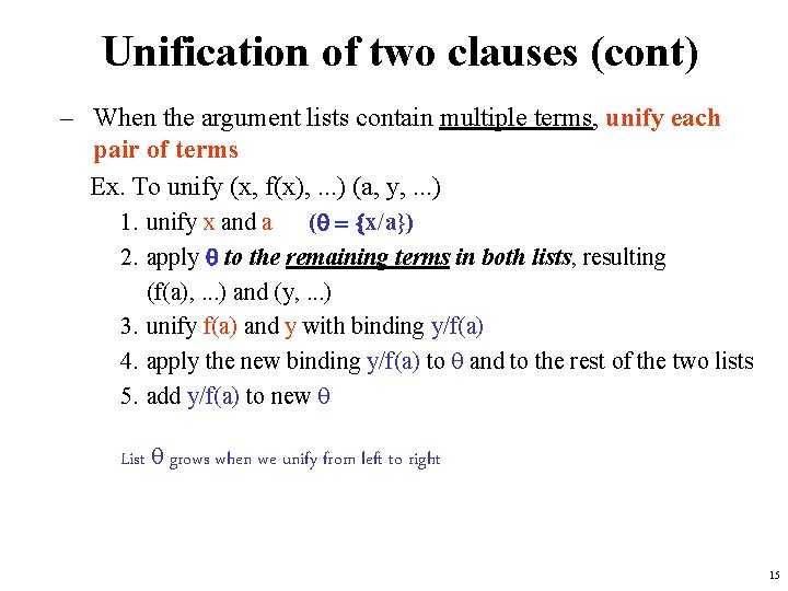
Unification of two clauses (cont) – When the argument lists contain multiple terms, unify each pair of terms Ex. To unify (x, f(x), . . . ) (a, y, . . . ) 1. unify x and a (q = {x/a}) 2. apply q to the remaining terms in both lists, resulting (f(a), . . . ) and (y, . . . ) 3. unify f(a) and y with binding y/f(a) 4. apply the new binding y/f(a) to q and to the rest of the two lists 5. add y/f(a) to new q List q grows when we unify from left to right 15

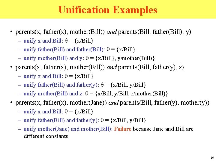
Unification Examples • parents(x, father(x), mother(Bill)) and parents(Bill, father(Bill), y) – unify x and Bill: q = {x/Bill} – unify father(Bill) and father(Bill): q = {x/Bill} – unify mother(Bill) and y: q = {x/Bill}, y/mother(Bill)} • parents(x, father(x), mother(Bill)) and parents(Bill, father(y), z) – unify x and Bill: q = {x/Bill} – unify father(Bill) and father(y): q = {x/Bill, y/Bill} – unify mother(Bill) and z: q = {x/Bill, y/Bill, z/mother(Bill)} • parents(x, father(x), mother(Jane)) and parents(Bill, father(y), mother(y)) – unify x and Bill: q = {x/Bill} – unify father(Bill) and father(y): q = {x/Bill, y/Bill} – unify mother(Jane) and mother(Bill): Failure because Jane and Bill are different constants 16

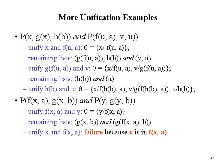
More Unification Examples • P(x, g(x), h(b)) and P(f(u, a), v, u)) – unify x and f(u, a): q = {x/ f(u, a)}; remaining lists: (g(f(u, a)), h(b)) and (v, u) – unify g(f(u, a)) and v: q = {x/f(u, a), v/g(f(u, a))}; remaining lists: (h(b)) and (u) – unify h(b) and u: q = {x/f(h(b), a), v/g(f(h(b), a)), u/h(b)}; • P(f(x, a), g(x, b)) and P(y, g(y, b)) – unify f(x, a) and y: q = {y/f(x, a)} remaining lists: (g(x, b)) and (g(f(x, a), b)) – unify x and f(x, a): failure because x is in f(x, a) 17

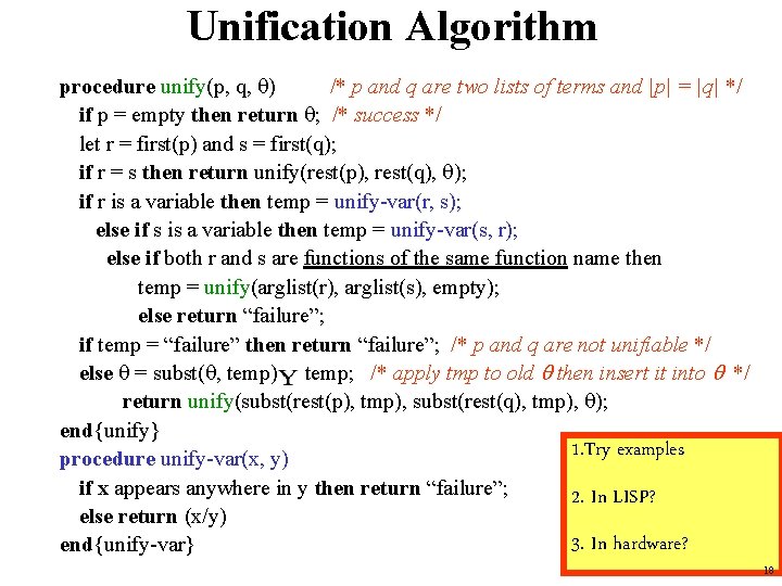
Unification Algorithm procedure unify(p, q, q) /* p and q are two lists of terms and |p| = |q| */ if p = empty then return q; /* success */ let r = first(p) and s = first(q); if r = s then return unify(rest(p), rest(q), q); if r is a variable then temp = unify-var(r, s); else if s is a variable then temp = unify-var(s, r); else if both r and s are functions of the same function name then temp = unify(arglist(r), arglist(s), empty); else return “failure”; if temp = “failure” then return “failure”; /* p and q are not unifiable */ else q = subst(q, temp) temp; /* apply tmp to old q then insert it into q */ return unify(subst(rest(p), tmp), subst(rest(q), tmp), q); end{unify} 1. Try examples procedure unify-var(x, y) if x appears anywhere in y then return “failure”; 2. In LISP? else return (x/y) 3. In hardware? end{unify-var} 18

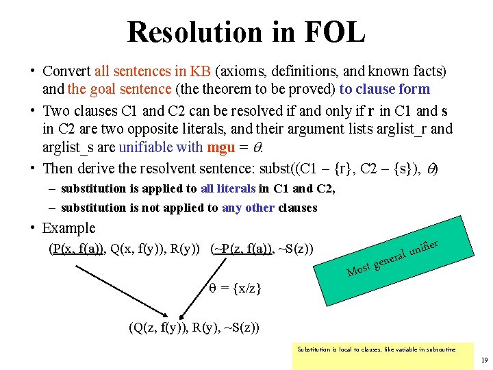
Resolution in FOL • Convert all sentences in KB (axioms, definitions, and known facts) and the goal sentence (the theorem to be proved) to clause form • Two clauses C 1 and C 2 can be resolved if and only if r in C 1 and s in C 2 are two opposite literals, and their argument lists arglist_r and arglist_s are unifiable with mgu = q. • Then derive the resolvent sentence: subst((C 1 – {r}, C 2 – {s}), q) – substitution is applied to all literals in C 1 and C 2, – substitution is not applied to any other clauses • Example ier f i n u eneral (P(x, f(a)), Q(x, f(y)), R(y)) (~P(z, f(a)), ~S(z)) q = {x/z} g Most (Q(z, f(y)), R(y), ~S(z)) Substitution is local to clauses, like variable in subroutine 19

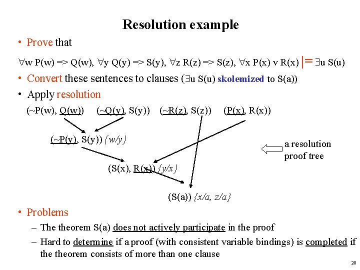
Resolution example • Prove that w P(w) => Q(w), y Q(y) => S(y), z R(z) => S(z), x P(x) v R(x) |= u S(u) • Convert these sentences to clauses ( u S(u) skolemized to S(a)) • Apply resolution (~P(w), Q(w)) (~Q(y), S(y)) (~R(z), S(z)) (P(x), R(x)) (~P(y), S(y)) {w/y} a resolution proof tree (S(x), R(x)) {y/x} (S(a)) {x/a, z/a} • Problems – The theorem S(a) does not actively participate in the proof – Hard to determine if a proof (with consistent variable bindings) is completed if theorem consists of more than one clause 20

Advanced Material – not mandatory in 2009 Also, we do not discuss this year hardware for unification and computer architectures for robotics as they are less important (they are in curriculum and on WWW page). New proof strategies Resolution Refutation: a better proof strategy 21

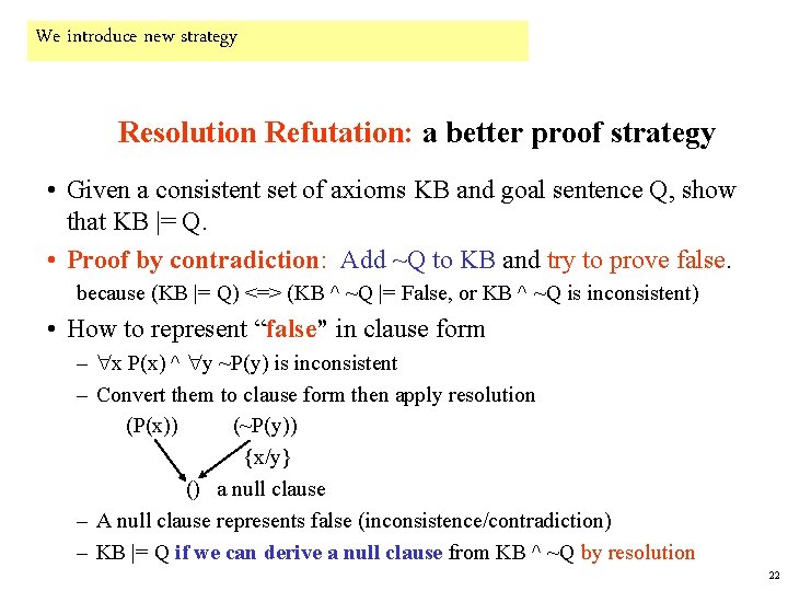
We introduce new strategy Resolution Refutation: a better proof strategy • Given a consistent set of axioms KB and goal sentence Q, show that KB |= Q. • Proof by contradiction: Add ~Q to KB and try to prove false. because (KB |= Q) <=> (KB ^ ~Q |= False, or KB ^ ~Q is inconsistent) • How to represent “false” in clause form – x P(x) ^ y ~P(y) is inconsistent – Convert them to clause form then apply resolution (P(x)) (~P(y)) {x/y} () a null clause – A null clause represents false (inconsistence/contradiction) – KB |= Q if we can derive a null clause from KB ^ ~Q by resolution 22

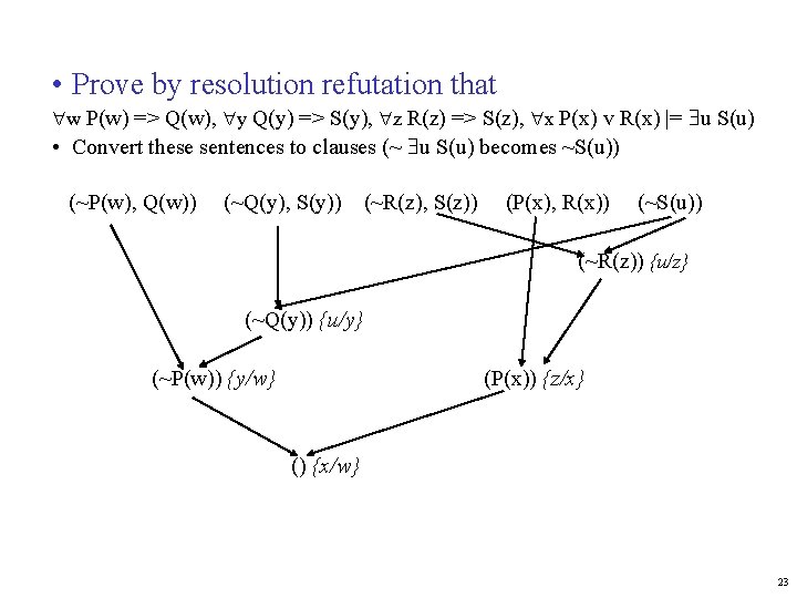
• Prove by resolution refutation that w P(w) => Q(w), y Q(y) => S(y), z R(z) => S(z), x P(x) v R(x) |= u S(u) • Convert these sentences to clauses (~ u S(u) becomes ~S(u)) (~P(w), Q(w)) (~Q(y), S(y)) (~R(z), S(z)) (P(x), R(x)) (~S(u)) (~R(z)) {u/z} (~Q(y)) {u/y} (~P(w)) {y/w} (P(x)) {z/x} () {x/w} 23

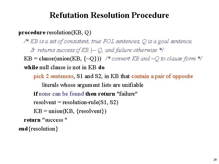
Refutation Resolution Procedure procedure resolution(KB, Q) /* KB is a set of consistent, true FOL sentences, Q is a goal sentence. It returns success if KB |-- Q, and failure otherwise */ KB = clause(union(KB, {~Q})) /* convert KB and ~Q to clause form */ while null clause is not in KB do pick 2 sentences, S 1 and S 2, in KB that contain a pair of opposite literals whose argument lists are unifiable if none can be found then return "failure" resolvent = resolution-rule(S 1, S 2) KB = union(KB, {resolvent}) return "success " end{resolution} 24

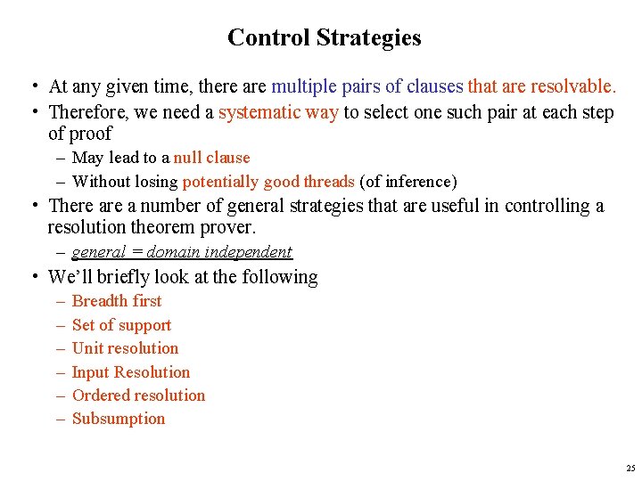
Control Strategies • At any given time, there are multiple pairs of clauses that are resolvable. • Therefore, we need a systematic way to select one such pair at each step of proof – May lead to a null clause – Without losing potentially good threads (of inference) • There a number of general strategies that are useful in controlling a resolution theorem prover. – general = domain independent • We’ll briefly look at the following – – – Breadth first Set of support Unit resolution Input Resolution Ordered resolution Subsumption 25

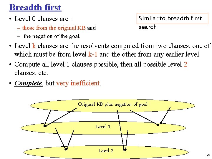
Breadth first • Level 0 clauses are : Similar to breadth first search – those from the original KB and – the negation of the goal. • Level k clauses are the resolvents computed from two clauses, one of which must be from level k-1 and the other from any earlier level. • Compute all level 1 clauses possible, then all possible level 2 clauses, etc. • Complete, but very inefficient. Original KB plus negation of goal Level 1 Level 2 26

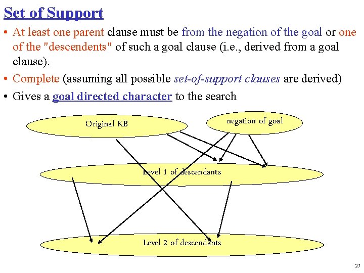
Set of Support • At least one parent clause must be from the negation of the goal or one of the "descendents" of such a goal clause (i. e. , derived from a goal clause). • Complete (assuming all possible set-of-support clauses are derived) • Gives a goal directed character to the search negation of goal Original KB Level 1 of descendants Level 2 of descendants 27

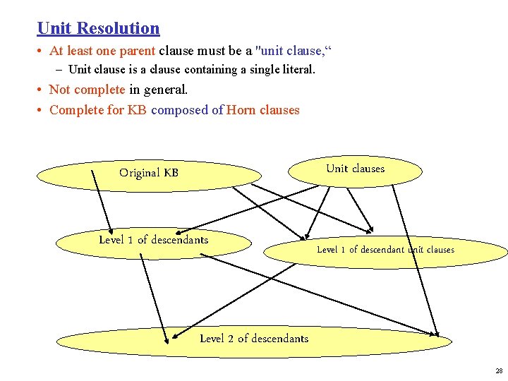
Unit Resolution • At least one parent clause must be a "unit clause, “ – Unit clause is a clause containing a single literal. • Not complete in general. • Complete for KB composed of Horn clauses Unit clauses Original KB Level 1 of descendants Level 1 of descendant unit clauses Level 2 of descendants 28

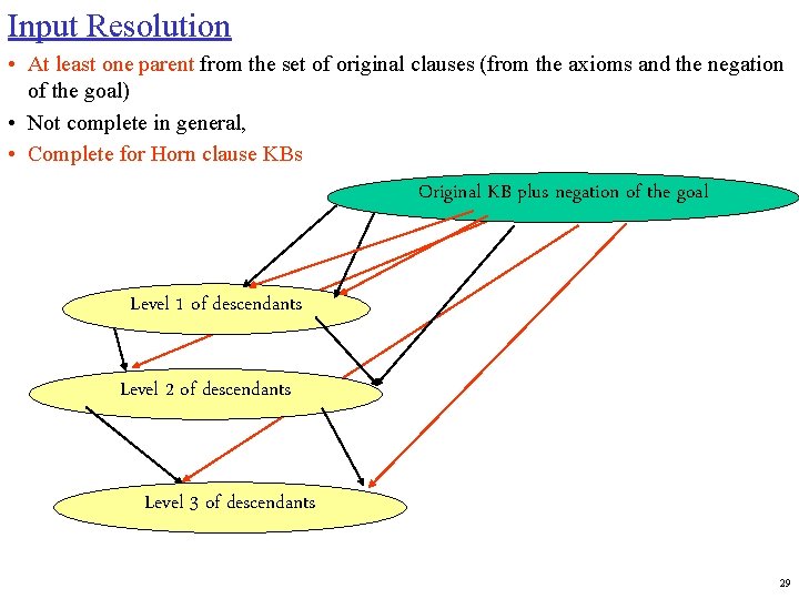
Input Resolution • At least one parent from the set of original clauses (from the axioms and the negation of the goal) • Not complete in general, • Complete for Horn clause KBs Original KB plus negation of the goal Level 1 of descendants Level 2 of descendants Level 3 of descendants 29

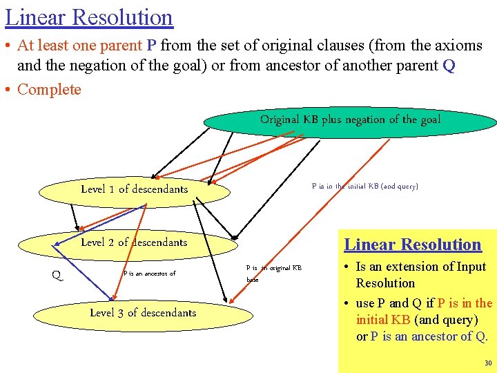
Linear Resolution • At least one parent P from the set of original clauses (from the axioms and the negation of the goal) or from ancestor of another parent Q • Complete Original KB plus negation of the goal P is in the initial KB (and query) Level 1 of descendants Linear Resolution Level 2 of descendants Q P is an ancestor of Level 3 of descendants P is in original KB base • Is an extension of Input Resolution • use P and Q if P is in the initial KB (and query) or P is an ancestor of Q. 30

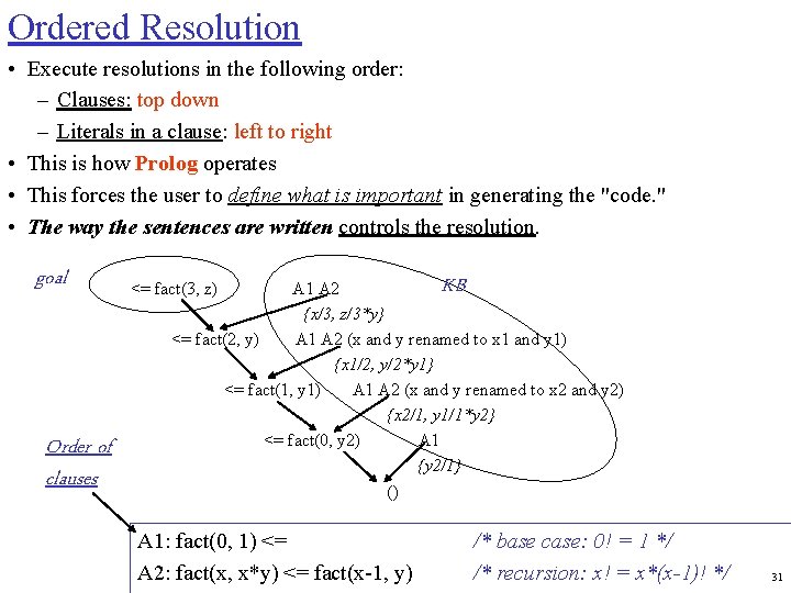
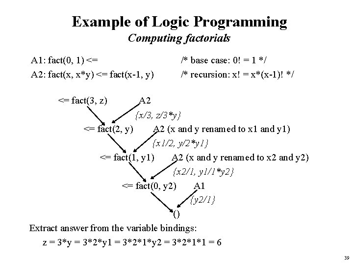
Ordered Resolution • Execute resolutions in the following order: – Clauses: top down – Literals in a clause: left to right • This is how Prolog operates • This forces the user to define what is important in generating the "code. " • The way the sentences are written controls the resolution. goal Order of clauses KB A 1 A 2 {x/3, z/3*y} <= fact(2, y) A 1 A 2 (x and y renamed to x 1 and y 1) {x 1/2, y/2*y 1} <= fact(1, y 1) A 1 A 2 (x and y renamed to x 2 and y 2) {x 2/1, y 1/1*y 2} <= fact(0, y 2) A 1 {y 2/1} () <= fact(3, z) A 1: fact(0, 1) <= A 2: fact(x, x*y) <= fact(x-1, y) /* base case: 0! = 1 */ /* recursion: x! = x*(x-1)! */ 31

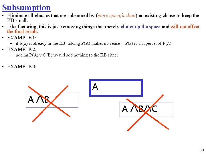
Subsumption • Eliminate all clauses that are subsumed by (more specific than) an existing clause to keep the KB small. • Like factoring, this is just removing things that merely clutter up the space and will not affect the final result. • EXAMPLE 1: – if P(x) is already in the KB, adding P(A) makes no sense -- P(x) is a superset of P(A). • EXAMPLE 2: – adding P(A) v Q(B) would add nothing to the KB either. • EXAMPLE 3: A A /B/C 32

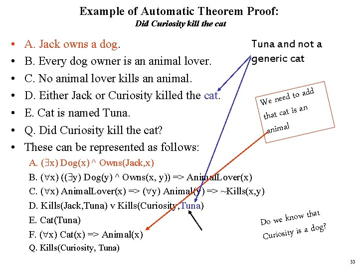
Example of Automatic Theorem Proof: Did Curiosity kill the cat • • A. Jack owns a dog. B. Every dog owner is an animal lover. C. No animal lover kills an animal. D. Either Jack or Curiosity killed the cat. E. Cat is named Tuna. Q. Did Curiosity kill the cat? These can be represented as follows: Tuna and not a generic cat add o t d e e We n an s i t a c t tha animal A. ( x) Dog(x) ^ Owns(Jack, x) B. ( x) (( y) Dog(y) ^ Owns(x, y)) => Animal. Lover(x) C. ( x) Animal. Lover(x) => ( y) Animal(y) => ~Kills(x, y) D. Kills(Jack, Tuna) v Kills(Curiosity, Tuna) that w o n k e w E. Cat(Tuna) Do g? o d a s i y t F. ( x) Cat(x) => Animal(x) Curiosi Q. Kills(Curiosity, Tuna) 33

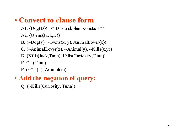
• Convert to clause form A 1. (Dog(D)) /* D is a skolem constant */ A 2. (Owns(Jack, D)) B. (~Dog(y), ~Owns(x, y), Animal. Lover(x)) C. (~Animal. Lover(x), ~Animal(y), ~Kills(x, y)) D. (Kills(Jack, Tuna), Kills(Curiosity, Tuna)) E. Cat(Tuna) F. (~Cat(x), Animal(x)) • Add the negation of query: Q: (~Kills(Curiosity, Tuna)) 34

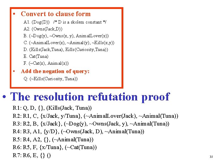
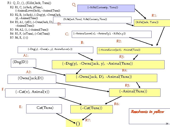
• Convert to clause form A 1. (Dog(D)) /* D is a skolem constant */ A 2. (Owns(Jack, D)) B. (~Dog(y), ~Owns(x, y), Animal. Lover(x)) C. (~Animal. Lover(x), ~Animal(y), ~Kills(x, y)) D. (Kills(Jack, Tuna), Kills(Curiosity, Tuna)) E. Cat(Tuna) F. (~Cat(x), Animal(x)) • Add the negation of query: Q: (~Kills(Curiosity, Tuna)) • The resolution refutation proof R 1: Q, D, {}, (Kills(Jack, Tuna)) R 2: R 1, C, {x/Jack, y/Tuna}, (~Animal. Lover(Jack), ~Animal(Tuna)) R 3: R 2, B, {x/Jack}, (~Dog(y), ~Owns(Jack, y), ~Animal(Tuna)) R 4: R 3, A 1, {y/D}, (~Owns(Jack, D), ~Animal(Tuna)) R 5: R 4, A 2, {}, (~Animal(Tuna)) R 6: R 5, F, {x/Tuna}, (~Cat(Tuna)) R 7: R 6, E, {} () 35

R 1: Q, D, {}, (Kills(Jack, Tuna)) R 2: R 1, C, {x/Jack, y/Tuna}, (~Animal. Lover(Jack), ~Animal(Tuna)) R 3: R 2, B, {x/Jack}, (~Dog(y), ~Owns(Jack, y), ~Animal(Tuna)) R 4: R 3, A 1, {y/D}, (~Owns(Jack, D), ~Animal(Tuna)) R 5: R 4, A 2, {}, (~Animal(Tuna)) R 6: R 5, F, {x/Tuna}, (~Cat(Tuna)) R 7: R 6, E, {} () D: Q: (~Kills(Curiosity, Tuna)) (Kills(Jack, Tuna), Kills(Curiosity, Tuna)) C: A 2: (Owns(Jack, D)) F: R 2: B: (~Animal. Lover(Jack), ~Animal(Tuna)) R 3: (~Dog(y), ~Owns(Jack, y), ~Animal(Tuna)) R 4: (~Owns(Jack, D), ~Animal(Tuna)) R 5: (~Animal(Tuna)) (~Cat(x), Animal(x)) E: (Kills(Jack, Tuna)) (~Animal. Lover(x), ~Animal(y), ~Kills(x, y)) (~Dog(y), ~Owns(x, y), Animal. Lover(x)) A 1: (Dog(D)) R 1: Cat(Tuna) (~Cat(Tuna)) () R 7: R 6: Resolvents in yellow 36

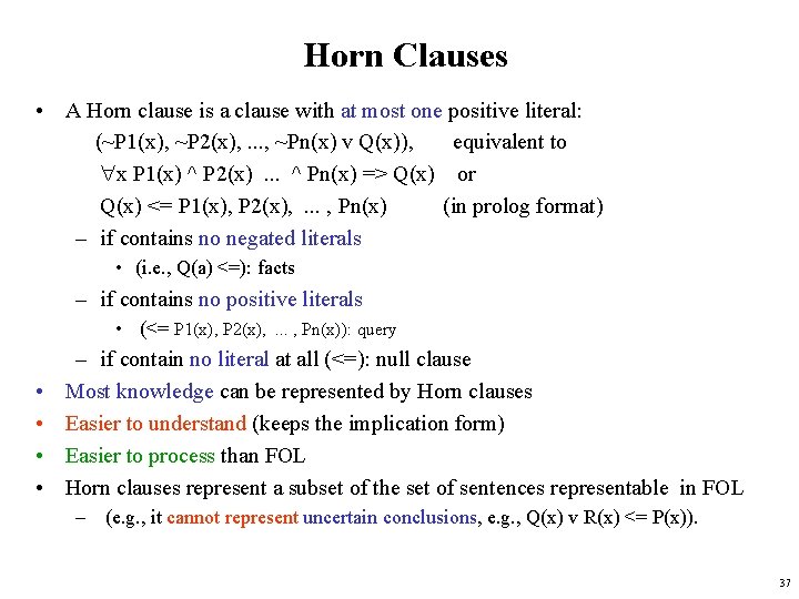
Horn Clauses • A Horn clause is a clause with at most one positive literal: (~P 1(x), ~P 2(x), . . . , ~Pn(x) v Q(x)), equivalent to x P 1(x) ^ P 2(x). . . ^ Pn(x) => Q(x) or Q(x) <= P 1(x), P 2(x), . . . , Pn(x) (in prolog format) – if contains no negated literals • (i. e. , Q(a) <=): facts – if contains no positive literals • (<= P 1(x), P 2(x), . . . , Pn(x)): query • • – if contain no literal at all (<=): null clause Most knowledge can be represented by Horn clauses Easier to understand (keeps the implication form) Easier to process than FOL Horn clauses represent a subset of the set of sentences representable in FOL – (e. g. , it cannot represent uncertain conclusions, e. g. , Q(x) v R(x) <= P(x)). 37

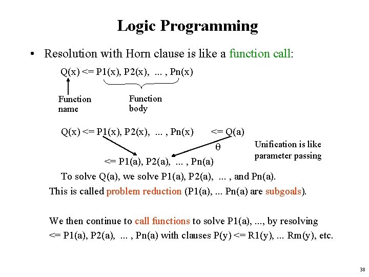
Logic Programming • Resolution with Horn clause is like a function call: Q(x) <= P 1(x), P 2(x), . . . , Pn(x) Function name Function body Q(x) <= P 1(x), P 2(x), . . . , Pn(x) <= Q(a) Unification is like q parameter passing <= P 1(a), P 2(a), . . . , Pn(a) To solve Q(a), we solve P 1(a), P 2(a), . . . , and Pn(a). This is called problem reduction (P 1(a), . . . Pn(a) are subgoals). We then continue to call functions to solve P 1(a), . . . , by resolving <= P 1(a), P 2(a), . . . , Pn(a) with clauses P(y) <= R 1(y), . . . Rm(y), etc. 38

Example of Logic Programming Computing factorials A 1: fact(0, 1) <= A 2: fact(x, x*y) <= fact(x-1, y) /* base case: 0! = 1 */ /* recursion: x! = x*(x-1)! */ <= fact(3, z) A 2 {x/3, z/3*y} <= fact(2, y) A 2 (x and y renamed to x 1 and y 1) {x 1/2, y/2*y 1} <= fact(1, y 1) A 2 (x and y renamed to x 2 and y 2) {x 2/1, y 1/1*y 2} <= fact(0, y 2) A 1 {y 2/1} () Extract answer from the variable bindings: z = 3*y = 3*2*y 1 = 3*2*1*y 2 = 3*2*1*1 = 6 39

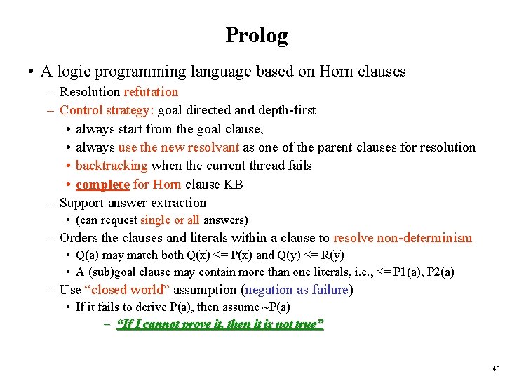
Prolog • A logic programming language based on Horn clauses – Resolution refutation – Control strategy: goal directed and depth-first • always start from the goal clause, • always use the new resolvant as one of the parent clauses for resolution • backtracking when the current thread fails • complete for Horn clause KB – Support answer extraction • (can request single or all answers) – Orders the clauses and literals within a clause to resolve non-determinism • Q(a) may match both Q(x) <= P(x) and Q(y) <= R(y) • A (sub)goal clause may contain more than one literals, i. e. , <= P 1(a), P 2(a) – Use “closed world” assumption (negation as failure) • If it fails to derive P(a), then assume ~P(a) – “If I cannot prove it, then it is not true” 40

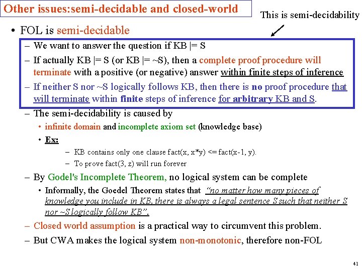
Other issues: semi-decidable and closed-world This is semi-decidability • FOL is semi-decidable – We want to answer the question if KB |= S – If actually KB |= S (or KB |= ~S), then a complete proof procedure will terminate with a positive (or negative) answer within finite steps of inference – If neither S nor ~S logically follows KB, then there is no proof procedure that will terminate within finite steps of inference for arbitrary KB and S. – The semi-decidability is caused by • infinite domain and incomplete axiom set (knowledge base) • Ex: – KB contains only one clause fact(x, x*y) <= fact(x-1, y). – To prove fact(3, z) will run forever – By Godel's Incomplete Theorem, no logical system can be complete • Informally, the Goedel Theorem states that “no matter how many pieces of knowledge you include in KB, there is always a legal sentence S such that neither S nor ~S logically follow KB”. – Closed world assumption is a practical way to circumvent this problem. – But CWA makes the logical system non-monotonic, therefore non-FOL 41

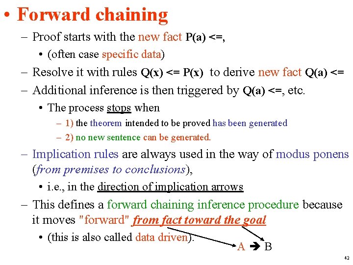
• Forward chaining – Proof starts with the new fact P(a) <=, • (often case specific data) – Resolve it with rules Q(x) <= P(x) to derive new fact Q(a) <= – Additional inference is then triggered by Q(a) <=, etc. • The process stops when – 1) theorem intended to be proved has been generated – 2) no new sentence can be generated. – Implication rules are always used in the way of modus ponens (from premises to conclusions), • i. e. , in the direction of implication arrows – This defines a forward chaining inference procedure because it moves "forward" from fact toward the goal • (this is also called data driven). A B 42

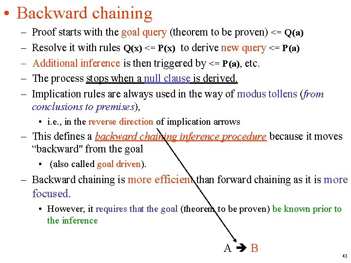
• Backward chaining – – – Proof starts with the goal query (theorem to be proven) <= Q(a) Resolve it with rules Q(x) <= P(x) to derive new query <= P(a) Additional inference is then triggered by <= P(a), etc. The process stops when a null clause is derived. Implication rules are always used in the way of modus tollens (from conclusions to premises), • i. e. , in the reverse direction of implication arrows – This defines a backward chaining inference procedure because it moves “backward" from the goal • (also called goal driven). – Backward chaining is more efficient than forward chaining as it is more focused. • However, it requires that the goal (theorem to be proven) be known prior to the inference A B 43