Inference in First Order Logic Some material adopted

Inference in First Order Logic Some material adopted from notes by Tim Finin, Andreas Geyer-Schulz, and Chuck Dyer 1

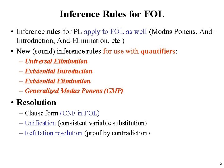
Inference Rules for FOL • Inference rules for PL apply to FOL as well (Modus Ponens, And. Introduction, And-Elimination, etc. ) • New (sound) inference rules for use with quantifiers: – Universal Elimination – Existential Introduction – Existential Elimination – Generalized Modus Ponens (GMP) • Resolution – Clause form (CNF in FOL) – Unification (consistent variable substitution) – Refutation resolution (proof by contradiction) 2

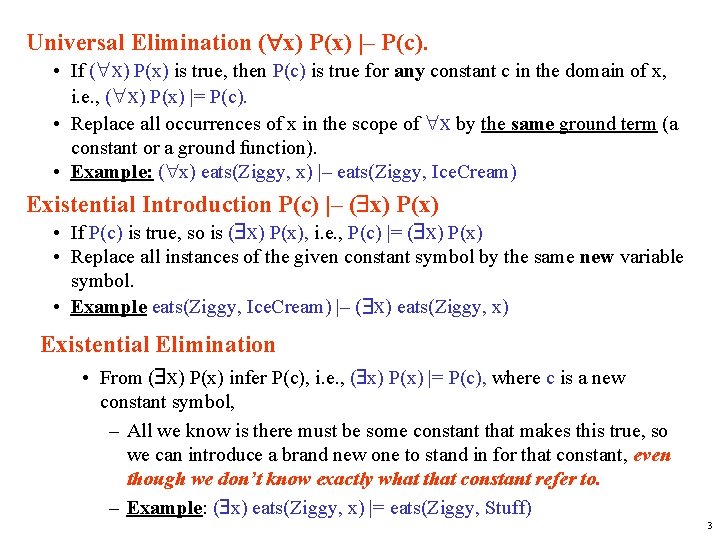
Universal Elimination ( x) P(x) |– P(c). • If ( x) P(x) is true, then P(c) is true for any constant c in the domain of x, i. e. , ( x) P(x) |= P(c). • Replace all occurrences of x in the scope of x by the same ground term (a constant or a ground function). • Example: ( x) eats(Ziggy, x) |– eats(Ziggy, Ice. Cream) Existential Introduction P(c) |– ( x) P(x) • If P(c) is true, so is ( x) P(x), i. e. , P(c) |= ( x) P(x) • Replace all instances of the given constant symbol by the same new variable symbol. • Example eats(Ziggy, Ice. Cream) |– ( x) eats(Ziggy, x) Existential Elimination • From ( x) P(x) infer P(c), i. e. , ( x) P(x) |= P(c), where c is a new constant symbol, – All we know is there must be some constant that makes this true, so we can introduce a brand new one to stand in for that constant, even though we don’t know exactly what that constant refer to. – Example: ( x) eats(Ziggy, x) |= eats(Ziggy, Stuff) 3

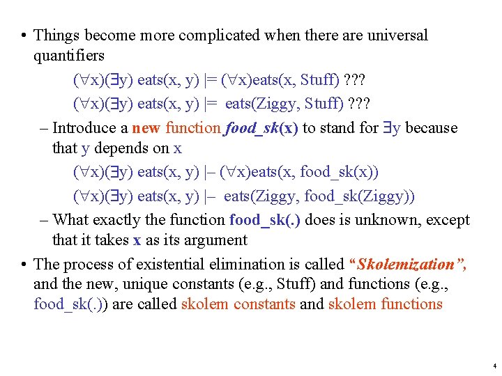
• Things become more complicated when there are universal quantifiers ( x)( y) eats(x, y) |= ( x)eats(x, Stuff) ? ? ? ( x)( y) eats(x, y) |= eats(Ziggy, Stuff) ? ? ? – Introduce a new function food_sk(x) to stand for y because that y depends on x ( x)( y) eats(x, y) |– ( x)eats(x, food_sk(x)) ( x)( y) eats(x, y) |– eats(Ziggy, food_sk(Ziggy)) – What exactly the function food_sk(. ) does is unknown, except that it takes x as its argument • The process of existential elimination is called “Skolemization”, and the new, unique constants (e. g. , Stuff) and functions (e. g. , food_sk(. )) are called skolem constants and skolem functions 4

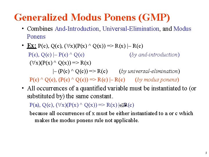
Generalized Modus Ponens (GMP) • Combines And-Introduction, Universal-Elimination, and Modus Ponens • Ex: P(c), Q(c), ( x)(P(x) ^ Q(x)) => R(x) |– R(c) P(c), Q(c) |– P(c) ^ Q(c) (by and-introduction) ( x)(P(x) ^ Q(x)) => R(x) |– (P(c) ^ Q(c)) => R(c) (by universal-elimination) P(c) ^ Q(c), (P(c) ^ Q(c)) => R(c) |– R(c) (by modus ponens) • All occurrences of a quantified variable must be instantiated to (or substituted by) the same constant. P(a), Q(c), ( x)(P(x) ^ Q(x)) => R(x) | – R(c) because all occurrences of x must be either instantiated to a or c which makes the modus ponens rule not applicable. 5

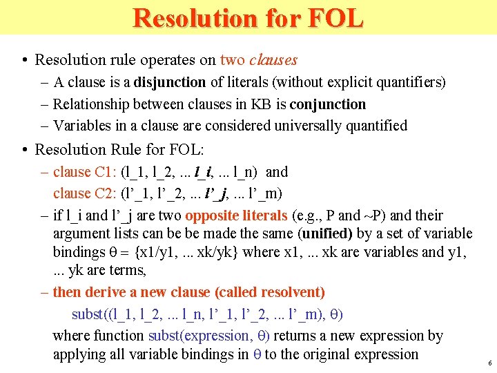
Resolution for FOL • Resolution rule operates on two clauses – A clause is a disjunction of literals (without explicit quantifiers) – Relationship between clauses in KB is conjunction – Variables in a clause are considered universally quantified • Resolution Rule for FOL: – clause C 1: (l_1, l_2, . . . l_i, . . . l_n) and clause C 2: (l’_1, l’_2, . . . l’_j, . . . l’_m) – if l_i and l’_j are two opposite literals (e. g. , P and ~P) and their argument lists can be be made the same (unified) by a set of variable bindings q = {x 1/y 1, . . . xk/yk} where x 1, . . . xk are variables and y 1, . . . yk are terms, – then derive a new clause (called resolvent) subst((l_1, l_2, . . . l_n, l’_1, l’_2, . . . l’_m), q) where function subst(expression, q) returns a new expression by applying all variable bindings in q to the original expression 6

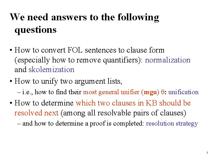
We need answers to the following questions • How to convert FOL sentences to clause form (especially how to remove quantifiers): normalization and skolemization • How to unify two argument lists, – i. e. , how to find their most general unifier (mgu) q: unification • How to determine which two clauses in KB should be resolved next (among all resolvable pairs of clauses) – and how to determine a proof is completed: resolution strategy 7

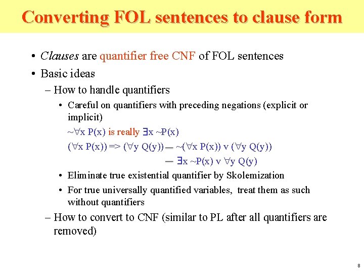
Converting FOL sentences to clause form • Clauses are quantifier free CNF of FOL sentences • Basic ideas – How to handle quantifiers • Careful on quantifiers with preceding negations (explicit or implicit) ~ x P(x) is really x ~P(x) ( x P(x)) => ( y Q(y)) ~( x P(x)) v ( y Q(y)) x ~P(x) v y Q(y) • Eliminate true existential quantifier by Skolemization • For true universally quantified variables, treat them as such without quantifiers – How to convert to CNF (similar to PL after all quantifiers are removed) 8

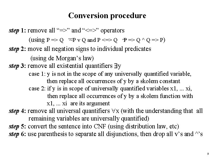
Conversion procedure step 1: remove all “=>” and “<=>” operators (using P => Q ~P v Q and P <=> Q P => Q ^ Q => P) step 2: move all negation signs to individual predicates (using de Morgan’s law) step 3: remove all existential quantifiers y case 1: y is not in the scope of any universally quantified variable, then replace all occurrences of y by a skolem constant case 2: if y is in scope of universally quantified variables x 1, . . . xi, then replace all occurrences of y by a skolem function with x 1, . . . xi are its argument step 4: remove all universal quantifiers x (with the understanding that all remaining variables are universally quantified) step 5: convert the sentence into CNF (using distribution law, etc) step 6: use parenthesis to separate all disjunctions, then drop all v’s and ^’s 9

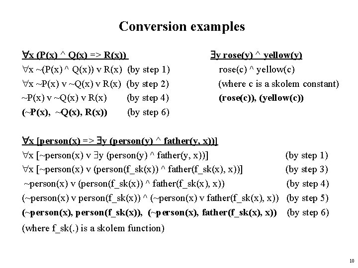
Conversion examples x (P(x) ^ Q(x) => R(x)) x ~(P(x) ^ Q(x)) v R(x) (by step 1) x ~P(x) v ~Q(x) v R(x) (by step 2) ~P(x) v ~Q(x) v R(x) (by step 4) (~P(x), ~Q(x), R(x)) (by step 6) y rose(y) ^ yellow(y) rose(c) ^ yellow(c) (where c is a skolem constant) (rose(c)), (yellow(c)) x [person(x) => y (person(y) ^ father(y, x))] x [~person(x) v (person(f_sk(x)) ^ father(f_sk(x), x))] ~person(x) v (person(f_sk(x)) ^ father(f_sk(x), x)) (~person(x) v person(f_sk(x)) ^ (~person(x) v father(f_sk(x), x)) (~person(x), person(f_sk(x)), (~person(x), father(f_sk(x), x)) (by step 1) (by step 3) (by step 4) (by step 5) (by step 6) (where f_sk(. ) is a skolem function) 10

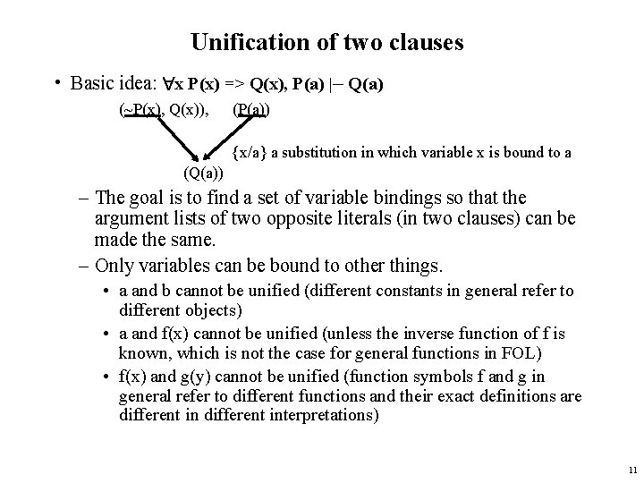
Unification of two clauses • Basic idea: x P(x) => Q(x), P(a) |– Q(a) (~P(x), Q(x)), (P(a)) {x/a} a substitution in which variable x is bound to a (Q(a)) – The goal is to find a set of variable bindings so that the argument lists of two opposite literals (in two clauses) can be made the same. – Only variables can be bound to other things. • a and b cannot be unified (different constants in general refer to different objects) • a and f(x) cannot be unified (unless the inverse function of f is known, which is not the case for general functions in FOL) • f(x) and g(y) cannot be unified (function symbols f and g in general refer to different functions and their exact definitions are different interpretations) 11

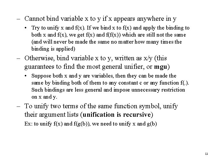
– Cannot bind variable x to y if x appears anywhere in y • Try to unify x and f(x). If we bind x to f(x) and apply the binding to both x and f(x), we get f(x) and f(f(x)) which are still not the same (and will never be made the same no matter how many times the binding is applied) – Otherwise, bind variable x to y, written as x/y (this guarantees to find the most general unifier, or mgu) • Suppose both x and y are variables, then they can be made the same by binding both of them to any constant c or any function f(. ). Such bindings are less general and impose unnecessary restriction on x and y. – To unify two terms of the same function symbol, unify their argument lists (unification is recursive) Ex: to unify f(x) and f(g(b)), we need to unify x and g(b) 12

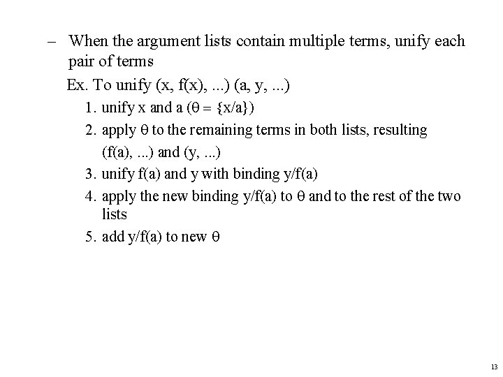
– When the argument lists contain multiple terms, unify each pair of terms Ex. To unify (x, f(x), . . . ) (a, y, . . . ) 1. unify x and a (q = {x/a}) 2. apply q to the remaining terms in both lists, resulting (f(a), . . . ) and (y, . . . ) 3. unify f(a) and y with binding y/f(a) 4. apply the new binding y/f(a) to q and to the rest of the two lists 5. add y/f(a) to new q 13

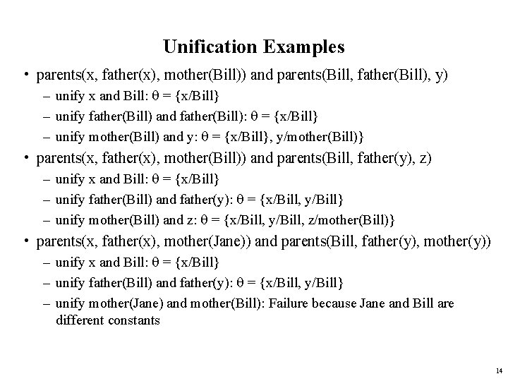
Unification Examples • parents(x, father(x), mother(Bill)) and parents(Bill, father(Bill), y) – unify x and Bill: q = {x/Bill} – unify father(Bill) and father(Bill): q = {x/Bill} – unify mother(Bill) and y: q = {x/Bill}, y/mother(Bill)} • parents(x, father(x), mother(Bill)) and parents(Bill, father(y), z) – unify x and Bill: q = {x/Bill} – unify father(Bill) and father(y): q = {x/Bill, y/Bill} – unify mother(Bill) and z: q = {x/Bill, y/Bill, z/mother(Bill)} • parents(x, father(x), mother(Jane)) and parents(Bill, father(y), mother(y)) – unify x and Bill: q = {x/Bill} – unify father(Bill) and father(y): q = {x/Bill, y/Bill} – unify mother(Jane) and mother(Bill): Failure because Jane and Bill are different constants 14

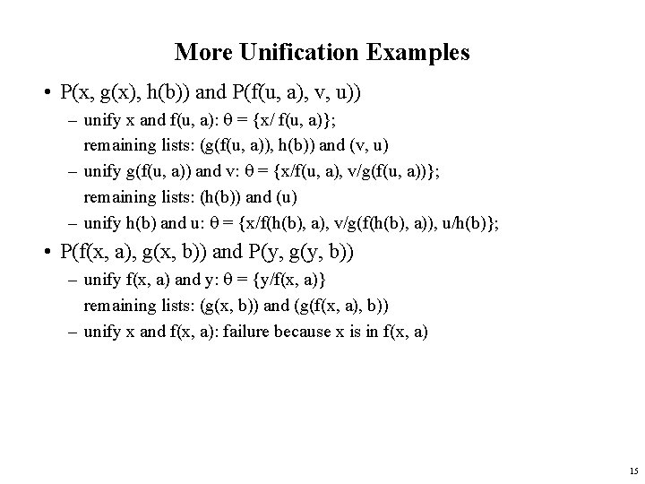
More Unification Examples • P(x, g(x), h(b)) and P(f(u, a), v, u)) – unify x and f(u, a): q = {x/ f(u, a)}; remaining lists: (g(f(u, a)), h(b)) and (v, u) – unify g(f(u, a)) and v: q = {x/f(u, a), v/g(f(u, a))}; remaining lists: (h(b)) and (u) – unify h(b) and u: q = {x/f(h(b), a), v/g(f(h(b), a)), u/h(b)}; • P(f(x, a), g(x, b)) and P(y, g(y, b)) – unify f(x, a) and y: q = {y/f(x, a)} remaining lists: (g(x, b)) and (g(f(x, a), b)) – unify x and f(x, a): failure because x is in f(x, a) 15

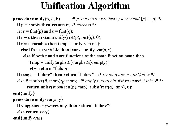
Unification Algorithm procedure unify(p, q, q) /* p and q are two lists of terms and |p| = |q| */ if p = empty then return q; /* success */ let r = first(p) and s = first(q); if r = s then return unify(rest(p), rest(q), q); if r is a variable then temp = unify-var(r, s); else if s is a variable then temp = unify-var(s, r); else if both r and s are functions of the same function name then temp = unify(arglist(r), arglist(s), empty); else return “failure”; if temp = “failure” then return “failure”; /* p and q are not unifiable */ else q = subst(q, temp) temp; /* apply tmp to old q then insert it into q */ return unify(subst(rest(p), tmp), subst(rest(q), tmp), q); end{unify} procedure unify-var(x, y) if x appears anywhere in y then return “failure”; else return (x/y) end{unify-var} 16

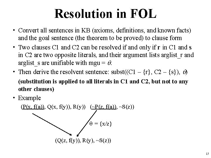
Resolution in FOL • Convert all sentences in KB (axioms, definitions, and known facts) and the goal sentence (the theorem to be proved) to clause form • Two clauses C 1 and C 2 can be resolved if and only if r in C 1 and s in C 2 are two opposite literals, and their argument lists arglist_r and arglist_s are unifiable with mgu = q. • Then derive the resolvent sentence: subst((C 1 – {r}, C 2 – {s}), q) (substitution is applied to all literals in C 1 and C 2, but not to any other clauses) • Example (P(x, f(a)), Q(x, f(y)), R(y)) (~P(z, f(a)), ~S(z)) q = {x/z} (Q(z, f(y)), R(y), ~S(z)) 17

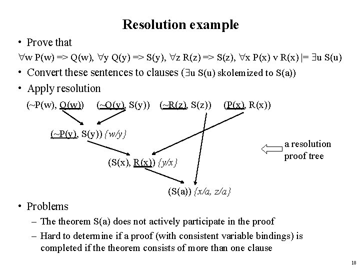
Resolution example • Prove that w P(w) => Q(w), y Q(y) => S(y), z R(z) => S(z), x P(x) v R(x) |= u S(u) • Convert these sentences to clauses ( u S(u) skolemized to S(a)) • Apply resolution (~P(w), Q(w)) (~Q(y), S(y)) (~R(z), S(z)) (P(x), R(x)) (~P(y), S(y)) {w/y} (S(x), R(x)) {y/x} a resolution proof tree (S(a)) {x/a, z/a} • Problems – The theorem S(a) does not actively participate in the proof – Hard to determine if a proof (with consistent variable bindings) is completed if theorem consists of more than one clause 18

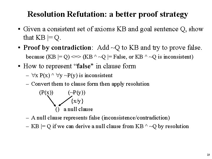
Resolution Refutation: a better proof strategy • Given a consistent set of axioms KB and goal sentence Q, show that KB |= Q. • Proof by contradiction: Add ~Q to KB and try to prove false. because (KB |= Q) <=> (KB ^ ~Q |= False, or KB ^ ~Q is inconsistent) • How to represent “false” in clause form – x P(x) ^ y ~P(y) is inconsistent – Convert them to clause form then apply resolution (P(x)) (~P(y)) {x/y} () a null clause – A null clause represents false (inconsistence/contradiction) – KB |= Q if we can derive a null clause from KB ^ ~Q by resolution 19

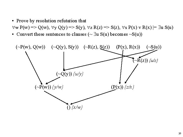
• Prove by resolution refutation that w P(w) => Q(w), y Q(y) => S(y), z R(z) => S(z), x P(x) v R(x) |= u S(u) • Convert these sentences to clauses (~ u S(u) becomes ~S(u)) (~P(w), Q(w)) (~Q(y), S(y)) (~R(z), S(z)) (P(x), R(x)) (~S(u)) (~R(z)) {u/z} (~Q(y)) {u/y} (~P(w)) {y/w} (P(x)) {z/x} () {x/w} 20

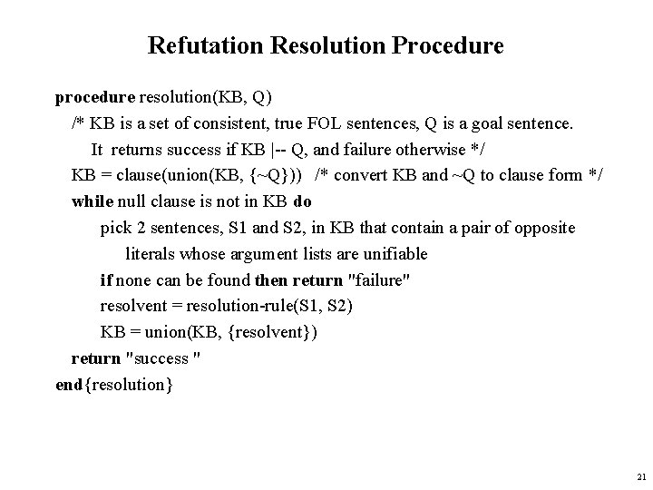
Refutation Resolution Procedure procedure resolution(KB, Q) /* KB is a set of consistent, true FOL sentences, Q is a goal sentence. It returns success if KB |-- Q, and failure otherwise */ KB = clause(union(KB, {~Q})) /* convert KB and ~Q to clause form */ while null clause is not in KB do pick 2 sentences, S 1 and S 2, in KB that contain a pair of opposite literals whose argument lists are unifiable if none can be found then return "failure" resolvent = resolution-rule(S 1, S 2) KB = union(KB, {resolvent}) return "success " end{resolution} 21

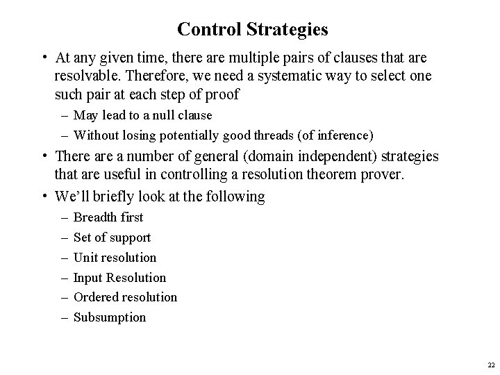
Control Strategies • At any given time, there are multiple pairs of clauses that are resolvable. Therefore, we need a systematic way to select one such pair at each step of proof – May lead to a null clause – Without losing potentially good threads (of inference) • There a number of general (domain independent) strategies that are useful in controlling a resolution theorem prover. • We’ll briefly look at the following – – – Breadth first Set of support Unit resolution Input Resolution Ordered resolution Subsumption 22

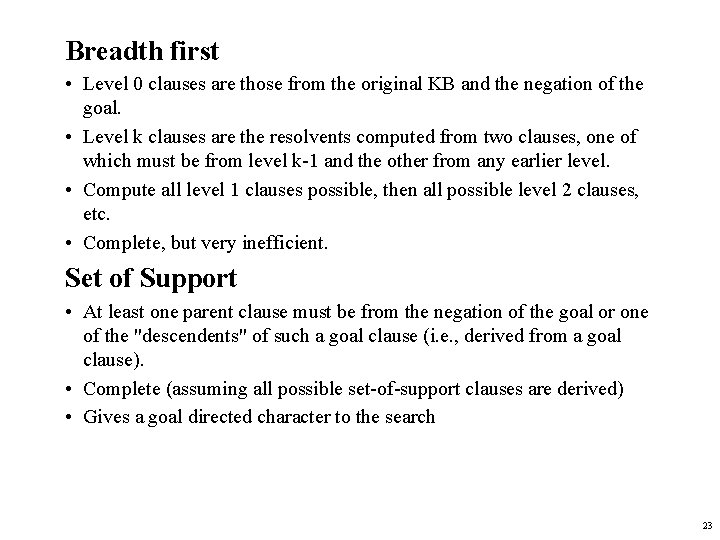
Breadth first • Level 0 clauses are those from the original KB and the negation of the goal. • Level k clauses are the resolvents computed from two clauses, one of which must be from level k-1 and the other from any earlier level. • Compute all level 1 clauses possible, then all possible level 2 clauses, etc. • Complete, but very inefficient. Set of Support • At least one parent clause must be from the negation of the goal or one of the "descendents" of such a goal clause (i. e. , derived from a goal clause). • Complete (assuming all possible set-of-support clauses are derived) • Gives a goal directed character to the search 23

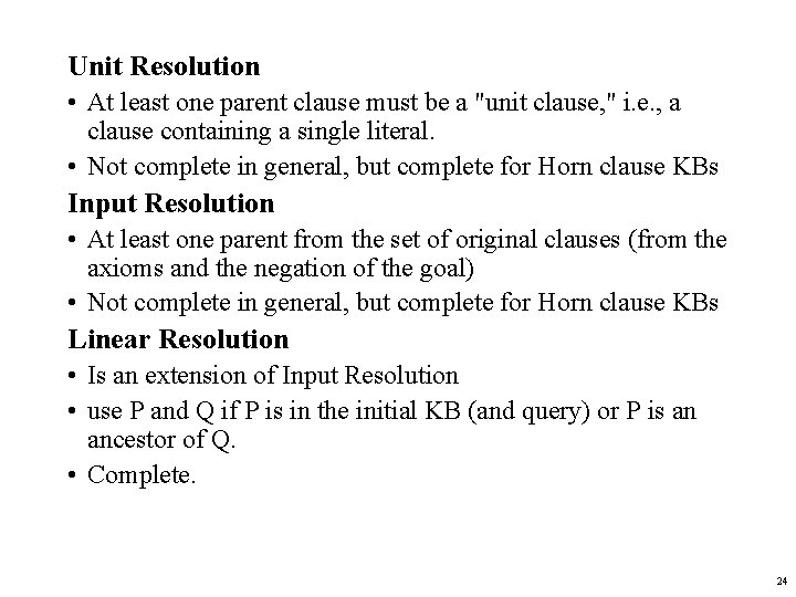
Unit Resolution • At least one parent clause must be a "unit clause, " i. e. , a clause containing a single literal. • Not complete in general, but complete for Horn clause KBs Input Resolution • At least one parent from the set of original clauses (from the axioms and the negation of the goal) • Not complete in general, but complete for Horn clause KBs Linear Resolution • Is an extension of Input Resolution • use P and Q if P is in the initial KB (and query) or P is an ancestor of Q. • Complete. 24

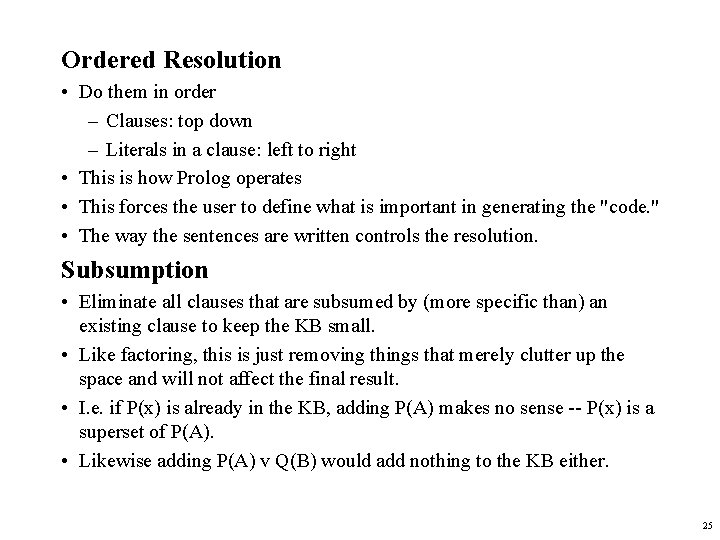
Ordered Resolution • Do them in order – Clauses: top down – Literals in a clause: left to right • This is how Prolog operates • This forces the user to define what is important in generating the "code. " • The way the sentences are written controls the resolution. Subsumption • Eliminate all clauses that are subsumed by (more specific than) an existing clause to keep the KB small. • Like factoring, this is just removing things that merely clutter up the space and will not affect the final result. • I. e. if P(x) is already in the KB, adding P(A) makes no sense -- P(x) is a superset of P(A). • Likewise adding P(A) v Q(B) would add nothing to the KB either. 25

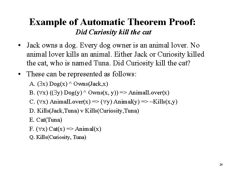
Example of Automatic Theorem Proof: Did Curiosity kill the cat • Jack owns a dog. Every dog owner is an animal lover. No animal lover kills an animal. Either Jack or Curiosity killed the cat, who is named Tuna. Did Curiosity kill the cat? • These can be represented as follows: A. ( x) Dog(x) ^ Owns(Jack, x) B. ( x) (( y) Dog(y) ^ Owns(x, y)) => Animal. Lover(x) C. ( x) Animal. Lover(x) => ( y) Animal(y) => ~Kills(x, y) D. Kills(Jack, Tuna) v Kills(Curiosity, Tuna) E. Cat(Tuna) F. ( x) Cat(x) => Animal(x) Q. Kills(Curiosity, Tuna) 26

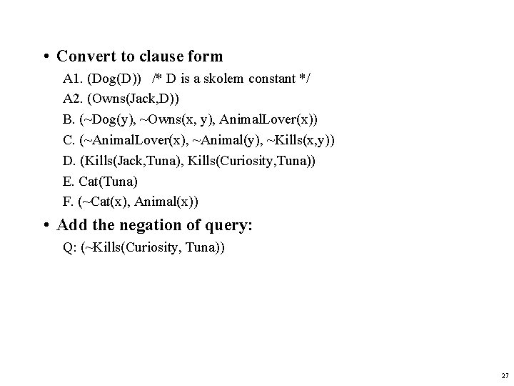
• Convert to clause form A 1. (Dog(D)) /* D is a skolem constant */ A 2. (Owns(Jack, D)) B. (~Dog(y), ~Owns(x, y), Animal. Lover(x)) C. (~Animal. Lover(x), ~Animal(y), ~Kills(x, y)) D. (Kills(Jack, Tuna), Kills(Curiosity, Tuna)) E. Cat(Tuna) F. (~Cat(x), Animal(x)) • Add the negation of query: Q: (~Kills(Curiosity, Tuna)) 27

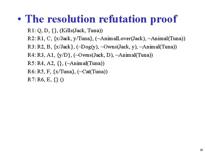
• The resolution refutation proof R 1: Q, D, {}, (Kills(Jack, Tuna)) R 2: R 1, C, {x/Jack, y/Tuna}, (~Animal. Lover(Jack), ~Animal(Tuna)) R 3: R 2, B, {x/Jack}, (~Dog(y), ~Owns(Jack, y), ~Animal(Tuna)) R 4: R 3, A 1, {y/D}, (~Owns(Jack, D), ~Animal(Tuna)) R 5: R 4, A 2, {}, (~Animal(Tuna)) R 6: R 5, F, {x/Tuna}, (~Cat(Tuna)) R 7: R 6, E, {} () 28

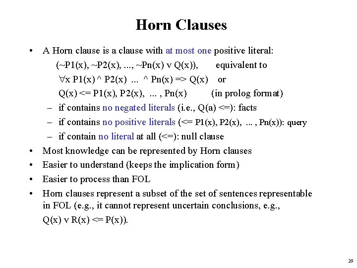
Horn Clauses • A Horn clause is a clause with at most one positive literal: (~P 1(x), ~P 2(x), . . . , ~Pn(x) v Q(x)), equivalent to x P 1(x) ^ P 2(x). . . ^ Pn(x) => Q(x) or Q(x) <= P 1(x), P 2(x), . . . , Pn(x) (in prolog format) – if contains no negated literals (i. e. , Q(a) <=): facts – if contains no positive literals (<= P 1(x), P 2(x), . . . , Pn(x)): query – if contain no literal at all (<=): null clause • Most knowledge can be represented by Horn clauses • Easier to understand (keeps the implication form) • Easier to process than FOL • Horn clauses represent a subset of the set of sentences representable in FOL (e. g. , it cannot represent uncertain conclusions, e. g. , Q(x) v R(x) <= P(x)). 29

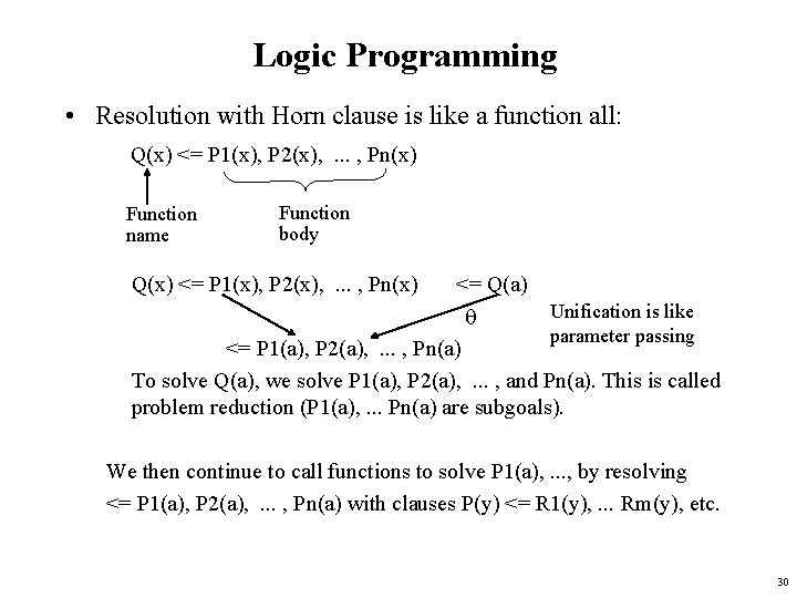
Logic Programming • Resolution with Horn clause is like a function all: Q(x) <= P 1(x), P 2(x), . . . , Pn(x) Function name Function body Q(x) <= P 1(x), P 2(x), . . . , Pn(x) <= Q(a) Unification is like q parameter passing <= P 1(a), P 2(a), . . . , Pn(a) To solve Q(a), we solve P 1(a), P 2(a), . . . , and Pn(a). This is called problem reduction (P 1(a), . . . Pn(a) are subgoals). We then continue to call functions to solve P 1(a), . . . , by resolving <= P 1(a), P 2(a), . . . , Pn(a) with clauses P(y) <= R 1(y), . . . Rm(y), etc. 30

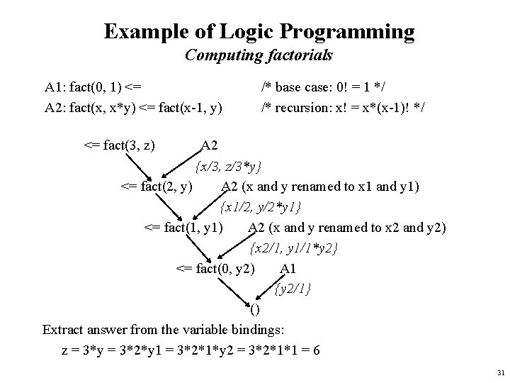
Example of Logic Programming Computing factorials A 1: fact(0, 1) <= A 2: fact(x, x*y) <= fact(x-1, y) /* base case: 0! = 1 */ /* recursion: x! = x*(x-1)! */ <= fact(3, z) A 2 {x/3, z/3*y} <= fact(2, y) A 2 (x and y renamed to x 1 and y 1) {x 1/2, y/2*y 1} <= fact(1, y 1) A 2 (x and y renamed to x 2 and y 2) {x 2/1, y 1/1*y 2} <= fact(0, y 2) A 1 {y 2/1} () Extract answer from the variable bindings: z = 3*y = 3*2*y 1 = 3*2*1*y 2 = 3*2*1*1 = 6 31

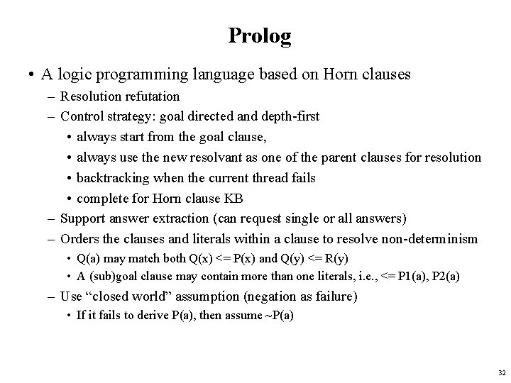
Prolog • A logic programming language based on Horn clauses – Resolution refutation – Control strategy: goal directed and depth-first • always start from the goal clause, • always use the new resolvant as one of the parent clauses for resolution • backtracking when the current thread fails • complete for Horn clause KB – Support answer extraction (can request single or all answers) – Orders the clauses and literals within a clause to resolve non-determinism • Q(a) may match both Q(x) <= P(x) and Q(y) <= R(y) • A (sub)goal clause may contain more than one literals, i. e. , <= P 1(a), P 2(a) – Use “closed world” assumption (negation as failure) • If it fails to derive P(a), then assume ~P(a) 32

Other issues • FOL is semi-decidable – We want to answer the question if KB |= S – If actually KB |= S (or KB |= ~S), then a complete proof procedure will terminate with a positive (or negative) answer within finite steps of inference – If neither S nor ~S logically follows KB, then there is no proof procedure will terminate within finite steps of inference for arbitrary KB and S. – The semi-decidability is caused by • infinite domain and incomplete axiom set (knowledge base) • Ex: KB contains only one clause fact(x, x*y) <= fact(x-1, y). To prove fact(3, z) will run forever – By Godel's Incomplete Theorem, no logical system can be complete (e. g. , no matter how many pieces of knowledge you include in KB, there is always a legal sentence S such that neither S nor ~S logically follow KB). – Closed world assumption is a practical way to circumvent this problem, but it make the logical system non-monotonic, therefore non-FOL 33

• Forward chaining – Proof starts with the new fact P(a) <=, (often case specific data) – Resolve it with rules Q(x) <= P(x) to derived new fact Q(a) <= – Additional inference is then triggered by Q(a) <=, etc. The process stops when theorem intended to proof (if there is one) has been generated or no new sentenced can be generated. – Implication rules are always used in the way of modus ponens (from premises to conclusions), i. e. , in the direction of implication arrows – This defines a forward chaining inference procedure because it moves "forward" from fact toward the goal (also called data driven). 34

• Backward chaining – Proof starts with the goal query (theorem to be proven) <= Q(a) – Resolve it with rules Q(x) <= P(x) to derived new query <= P(a) – Additional inference is then triggered by <= P(a), etc. The process stops when a null clause is derived. – Implication rules are always used in the way of modus tollens (from conclusions to premises), i. e. , in the reverse direction of implication arrows – This defines a backward chaining inference procedure because it moves “backward" from the goal (also called goal driven). – Backward chaining is more efficient than forward chaining as it is more focused. However, it requires that the goal (theorem to be proven) be known prior to the inference 35