Unit II First Order Logic SYNTAX AND SEMANTICS

Unit II First Order Logic

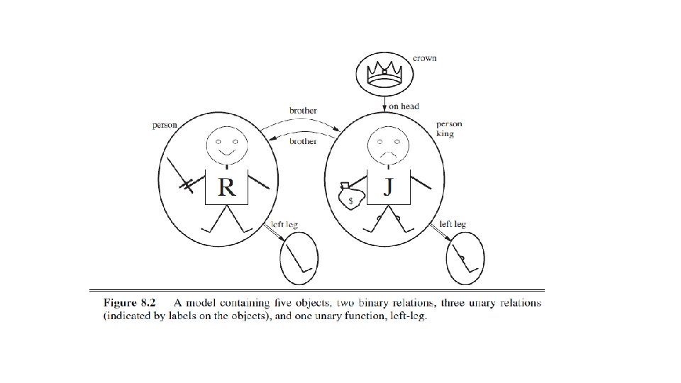
SYNTAX AND SEMANTICS OF FIRST-ORDER LOGIC – Models for First-Order Logic • The models of a logical language are the formal structures that constitute the possible worlds under consideration. • Each model links the vocabulary of the logical sentences to elements of the possible world, so that the truth of any sentence can be determined. • Thus, models for propositional logic link proposition symbols to predefined truth values. • Models for first-order logic have objects in them! • The domain of a model is the set of objects or domain elements it contains. • The domain is required to be nonempty—every possible world must contain at least one object. • Figure 8. 2 shows a model with five objects: Richard the Lionheart, King of England from 1189 to 1199; his younger brother, the evil King John, who ruled from 1199 to 1215; the left legs of Richard and John; and a crown.

• The objects in the model may be related in various ways. In the figure, Richard and John are brothers. • Formally speaking, a relation is just the set of tuples of objects that are related. (A tuple is a collection of objects arranged in a fixed order and is written with angle brackets surrounding the objects. ) • Thus, the brotherhood relation in this model is the set { (Richard the Lionheart, King John), (King John, Richard the Lionheart) }. (8. 1) • The crown is on King John’s head, so the “on head” relation contains just one tuple, the crown, King John. • The “brother” and “on head” relations are binary relations—that is, they relate pairs of objects. • The model also contains unary relations, or properties: the “person” property is true of both Richard and John; the “king” property is true only of John (presumably because Richard is dead at this point); and the “crown” property is true only of the crown. • Certain kinds of relationships are best considered as functions, in that a given object must be related to exactly one object in this way. • For example, each person has one left leg, so the model has a unary “left leg” function that includes the following mappings:

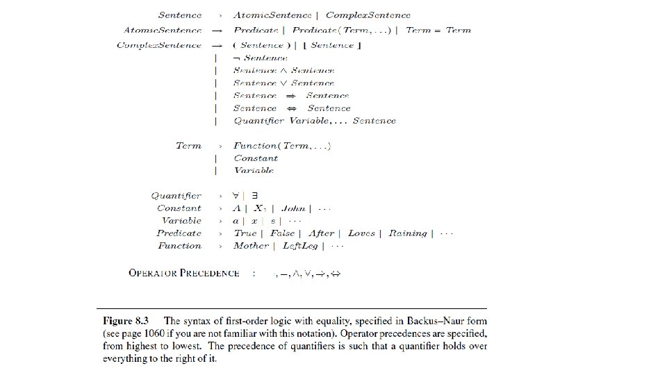
• Models in first-order logic require total functions, that is, there must be a value for every input tuple. • Thus, the crown must have a left leg and so must each of the left legs. • There is a technical solution to this awkward problem involving an additional “invisible” object that is the left leg of everything that has no left leg, including itself. • Fortunately, as long as one makes no assertions about the left legs of things that have no left legs, these technicalities are of no import. 2. Symbols and interpretations • The impatient reader can obtain a complete description from the formal grammar in Figure 8. 3. • The basic syntactic elements of first-order logic are the symbols that stand for objects, relations, and functions. • The symbols, therefore, come in three kinds: constant symbols, which stand for objects; predicate symbols, which stand for relations; and function symbols, which stand for functions. • We adopt the convention that these symbols will begin with uppercase letters. • For example, we might use the constant symbols Richard and John; the predicate symbols Brother , On. Head, Person, King, and Crown; and the function symbol Left. Leg. • As with proposition symbols, the choice of names is entirely up to the user. • Each predicate and function symbol comes with an arity that fixes the number of arguments.

• As in propositional logic, every model must provide the information required to determine if any given sentence is true or false. • Thus, in addition to its objects, relations, and functions, each model includes an interpretation that specifies exactly which objects, relations and functions are referred to by the constant, predicate, and function symbols. • One possible interpretation for our example—which a logician would call the intended interpretation—is as follows: § Richard refers to Richard the Lionheart and John refers to the evil King John. § Brother refers to the brotherhood relation, that is, the set of tuples of objects given in Equation (8. 1); On Head refers to the “on head” relation that holds between the crown and King John; Person, King, and Crown refer to the sets of objects that are persons, kings, and crowns. § Left. Leg refers to the “left leg” function, that is, the mapping given in Equation (8. 2). • There are many other possible interpretations, of course. For example, one interpretation maps Richard to the crown and John to King John’s left leg. • There are five objects in the model, so there are 25 possible interpretations just for the constant symbols Richard and John.

• It is also possible for an object to have several names; there is an interpretation under which both Richard and John refer to the crown. • If you find this possibility confusing, remember that, in propositional logic, it is perfectly possible to have a model in which Cloudy and Sunny are both true; it is the job of the knowledge base to rule out models that are inconsistent with our knowledge. • In summary, a model in first-order logic consists of a set of objects and an interpretation that maps constant symbols to objects, predicate symbols to relations on those objects, and function symbols to functions on those objects. • Just as with propositional logic, entailment, validity, and so on are defined in terms of all possible models. • To get an idea of what the set of all possible models looks like, see Figure 8. 4. • It shows that models vary in how many objects they contain—from one up to infinity— and in the way the constant symbols map to objects. • If there are two constant symbols and one object, then both symbols must refer to the same object; but this can still happen even with more objects. • When there are more objects than constant symbols, some of the objects will have no names.

• Because the number of possible models is unbounded, checking entailment by the enumeration of all possible models is not feasible for first-order logic (unlike propositional logic). • Even if the number of objects is restricted, the number of combinations can be very large. • For the example in Figure 8. 4, there are 137, 506, 194, 466 models with six or fewer objects.

3. Terms • A term is a logical expression that refers to an object. • Constant symbols are therefore terms, but it is not always convenient to have a distinct symbol to name every object. • For example, in English we might use the expression “King John’s left leg” rather than giving a name to his leg. • This is what function symbols are for: instead of using a constant symbol, we use Left. Leg(John). • In the general case, a complex term is formed by a function symbol followed by a parenthesized list of terms as arguments to the function symbol. • It is important to remember that a complex term is just a complicated kind of name. • It is not a “subroutine call” that “returns a value. ” • There is no Left. Leg subroutine that takes a person as input and returns a leg. • This is something that cannot be done with subroutines in programming languages

• The formal semantics of terms is straightforward. Consider a term f(t 1, . . . , tn). • The function symbol f refers to some function in the model (call it F); the argument terms refer to objects in the domain (call them d 1, . . . , dn); and the term as a whole refers to the object that is the value of the function F applied to d 1, . . . , dn. • For example, suppose the Left. Leg function symbol refers to the function shown in Equation (8. 2) and John refers to King John, then Left. Leg(John) refers to King John’s left leg. • In this way, the interpretation fixes the referent of every term. 4. Atomic sentences • An atomic sentence (or atom for short) is formed from a predicate symbol optionally followed by a parenthesized list of terms, such as Brother (Richard , John). • This states, under the intended interpretation given earlier, that Richard the Lionheart is the brother of King John. • Atomic sentences can have complex terms as arguments. Thus, Married(Father (Richard), Mother (John)) states that Richard the Lionheart’s father is married to King John’s mother. • An atomic sentence is true in a given model if the relation referred to by the predicate symbol holds among the objects referred to by the arguments.

5. Complex sentences • We can use logical connectives to construct more complex sentences, with the same syntax and semantics as in propositional calculus. Here are four sentences that are true in the model of Figure 8. 2 under our intended interpretation: ￢Brother (Left. Leg(Richard), John) Brother (Richard , John) ∧ Brother (John, Richard) King(Richard ) ∨ King(John) ￢King(Richard) ⇒ King(John). 6. Quantifiers • Once we have a logic that allows objects, it is only natural to want to express properties of entire collections of objects, instead of enumerating the objects by name. • Quantifiers let us do this. First-order logic contains two standard quantifiers, called universal and existential. Universal quantification (∀ - for all) • Rules such as “Squares neighboring the wumpus are smelly” and “All kings are persons” are the bread and butter of first-order logic. • The second rule, “All kings are persons, ” is written in first-order logic as ∀ x King(x) ⇒ Person(x). ∀ is usually pronounced “For all. . . ”. • Thus, the sentence says, “For all x, if x is a king, then x is a person. ”

• The symbol x is called a variable. By convention, variables are lowercase letters. • A variable is a term all by itself, and as such can also serve as the argument of a function—for example, Left. Leg(x). • A term with no variables is called a ground term. • Intuitively, the sentence ∀x P, where P is any logical expression, says that P is true for every object x. • More precisely, ∀x P is true in a given model if P is true in all possible extended interpretations constructed from the interpretation given in the model, where each extended interpretation specifies a domain element to which x refers. • This sounds complicated, but it is really just a careful way of stating the intuitive meaning of universal quantification. • Consider the model shown in Figure 8. 2 and the intended interpretation that goes with it. We can extend the interpretation in five ways: x → Richard the Lionheart, x → King John, x → Richard’s left leg, x → John’s left leg, x → the crown.

• The universally quantified sentence ∀ x King(x) ⇒ Person(x) is true in the original model if the sentence King(x) ⇒ Person(x) is true under each of the five extended interpretations. • That is, the universally quantified sentence is equivalent to asserting the following five sentences: Richard the Lionheart is a king ⇒ Richard the Lionheart is a person. King John is a king ⇒ King John is a person. Richard’s left leg is a king ⇒ Richard’s left leg is a person. John’s left leg is a king ⇒ John’s left leg is a person. The crown is a king ⇒ the crown is a person. • Let us look carefully at this set of assertions. Since, in our model, King John is the only king, the second sentence asserts that he is a person, as we would hope. • But what about the other four sentences, which appear to make claims about legs and crowns? • Is that part of the meaning of “All kings are persons”? In fact, the other four assertions are true in the model, but make no claim whatsoever about the personhood qualifications of legs, crowns, or indeed Richard. • Thus, the truth-table definition of ⇒ turns out to be perfect for writing general rules with universal quantifiers.

• A common mistake, made frequently even by diligent readers who have read this paragraph several times, is to use conjunction instead of implication. The sentence ∀ x King(x) ∧ Person(x) • would be equivalent to asserting Richard the Lionheart is a king ∧ Richard the Lionheart is a person, King John is a king ∧ King John is a person, Richard’s left leg is a king ∧ Richard’s left leg is a person, • and so on. Obviously, this does not capture what we want. Existential quantification (∃ - there exists or for some or there is at least one) • Universal quantification makes statements about every object. Similarly, we can make a statement about some object in the universe without naming it, by using an existential quantifier. • To say, for example, that King John has a crown on his head, we write ∃ x Crown(x) ∧ On. Head(x, John). • ∃x is pronounced “There exists an x such that. . . ” or “For some x. . . ”. • Intuitively, the sentence ∃ x P says that P is true for at least one object x. • More precisely, ∃ x P is true in a given model if P is true in at least one extended interpretation that assigns x to a domain element.

• That is, at least one of the following is true: Richard the Lionheart is a crown ∧ Richard the Lionheart is on John’s head; King John is a crown ∧ King John is on John’s head; Richard’s left leg is a crown ∧ Richard’s left leg is on John’s head; John’s left leg is a crown ∧ John’s left leg is on John’s head; The crown is a crown ∧ the crown is on John’s head. • The fifth assertion is true in the model, so the original existentially quantified sentence is true in the model. • Notice that, by our definition, the sentence would also be true in a model in which King John was wearing two crowns. • This is entirely consistent with the original sentence “King John has a crown on his head. ” • Just as ⇒ appears to be the natural connective to use with ∀, ∧ is the natural connective to use with ∃. • Using ∧ as the main connective with ∀ led to an overly strong statement in the example in the previous section; using ⇒ with ∃ usually leads to a very weak statement, indeed. • Consider the following sentence: ∃ x Crown(x) ⇒ On. Head(x, John).

• On the surface, this might look like a reasonable rendition of our sentence. • Applying the semantics, we see that the sentence says that at least one of the following assertions is true: Richard the Lionheart is a crown ⇒ Richard the Lionheart is on John’s head; King John is a crown ⇒ King John is on John’s head; Richard’s left leg is a crown ⇒ Richard’s left leg is on John’s head; • and so on. Now an implication is true if both premise and conclusion are true, or if its premise is false. • So if Richard the Lionheart is not a crown, then the first assertion is true and the existential is satisfied. Nested quantifiers • We will often want to express more complex sentences using multiple quantifiers. The simplest case is where the quantifiers are of the same type. For example, “Brothers are siblings” can be written as ∀ x ∀ y Brother (x, y) ⇒ Sibling(x, y).

• Consecutive quantifiers of the same type can be written as one quantifier with several variables. • For example, to say that siblinghood is a symmetric relationship, we can write ∀ x, y Sibling(x, y) ⇔ Sibling(y, x). • In other cases we will have mixtures. “Everybody loves somebody” means that for every person, there is someone that person loves: ∀x ∃ y Loves(x, y). • On the other hand, to say “There is someone who is loved by everyone, ” we write ∃ y ∀ x Loves(x, y). • The order of quantification is therefore very important. It becomes clearer if we insert parentheses. • ∀ x (∃ y Loves(x, y)) says that everyone has a particular property, namely, the property that they love someone. • On the other hand, ∃ y (∀ x Loves(x, y)) says that someone in the world has a particular property, namely the property of being loved by everybody. • Some confusion can arise when two quantifiers are used with the same variable name.

• Consider the sentence ∀ x (Crown(x) ∨ (∃ x Brother (Richard, x))). • Here the x in Brother (Richard, x) is existentially quantified. The rule is that the variable belongs to the innermost quantifier that mentions it; then it will not be subject to any other quantification. • Another way to think of it is this: ∃ x Brother (Richard, x) is a sentence about Richard (that he has a brother), not about x; so putting a ∀ x outside it has no effect. Connections between ∀ and ∃ • The two quantifiers are actually intimately connected with each other, through negation. • Asserting that everyone dislikes parsnips is the same as asserting there does not exist someone who likes them, and vice versa: ∀ x ￢Likes(x, Parsnips ) is equivalent to ￢∃ x Likes(x, Parsnips). • We can go one step further: “Everyone likes ice cream” means that there is no one who does not like ice cream: ∀ x Likes(x, Ice. Cream) is equivalent to ￢∃ x ￢Likes(x, Ice. Cream).

• Because ∀ is really a conjunction over the universe of objects and ∃ is a disjunction, it should not be surprising that they obey De Morgan’s rules. • The De Morgan rules for quantified and unquantified sentences are as follows: ∀ x ￢P ≡ ￢∃ x P ￢(P ∨ Q) ≡ ￢P ∧ ￢Q ￢∀ x P ≡ ∃ x ￢P ￢(P ∧ Q) ≡ ￢P ∨ ￢Q ∀ x P ≡ ￢∃ x ￢P P ∧ Q ≡ ￢(￢P ∨ ￢Q) ∃ x P ≡ ￢∀ x ￢P P ∨ Q ≡ ￢(￢P ∧ ￢Q) 7. Equality • First-order logic includes one more way to make atomic sentences, other than using a predicate and terms as described earlier. We can use the equality symbol to signify that two terms refer to the same object. For example, Father (John)=Henry • says that the object referred to by Father (John) and the object referred to by Henry are the same. • Because an interpretation fixes the referent of any term, determining the truth of an equality sentence is simply a matter of seeing that the referents of the two terms are the same object.

• The equality symbol can be used to state facts about a given function, as we just did for the Father symbol. • It can also be used with negation to insist that two terms are not the same object. • To say that Richard has at least two brothers, we would write ∃ x, y Brother (x, Richard) ∧ Brother (y, Richard) ∧ ￢(x=y). • The sentence ∃ x, y Brother (x, Richard) ∧ Brother (y, Richard) • does not have the intended meaning. • In particular, it is true in the model of Figure 8. 2, where Richard has only one brother. • To see this, consider the extended interpretation in which both x and y are assigned to King John. The addition of ￢(x=y) rules out such models. • The notation x ≠ y is sometimes used as an abbreviation for ￢(x=y).

8. An alternative semantics? • Continuing the example from the previous section, suppose that we believe that Richard has two brothers, John and Geoffrey. • Can we capture this state of affairs by asserting Brother (John, Richard) ∧ Brother (Geoffrey, Richard) ? (8. 3) • Not quite. First, this assertion is true in a model where Richard has only one brother— we need to add John ≠ Geoffrey. • Second, the sentence doesn’t rule out models in which Richard has many more brothers besides John and Geoffrey. • Thus, the correct translation of “Richard’s brothers are John and Geoffrey” is as follows: Brother (John, Richard) ∧ Brother (Geoffrey, Richard) ∧ John ≠ Geoffrey ∧ ∀ x Brother (x, Richard) ⇒ (x=John ∨ x=Geoffrey). • For many purposes, this seems much more cumbersome than the corresponding natural language expression. • As a consequence, humans may make mistakes in translating their knowledge into first-order logic, resulting in unintuitive behaviors from logical reasoning systems that use the knowledge.

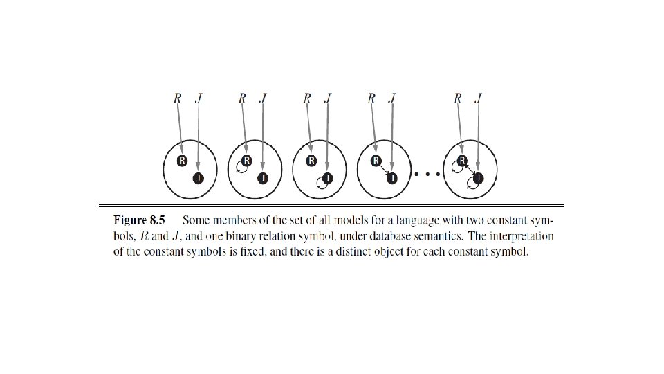
• One proposal that is very popular in database systems works as follows. • First, we insist that every constant symbol refer to a distinct object—the so-called unique-names assumption. • Second, we assume that atomic sentences not known to be true are in fact false—the closed-world assumption. • Finally, we invoke domain closure, meaning that each model contains no more domain elements than those named by the constant symbols. • Under the resulting semantics, which we call database semantics to distinguish it from the standard semantics of first-order logic, the sentence Equation (8. 3) does indeed state that Richard’s two brothers are John and Geoffrey. • It is instructive to consider the set of all possible models under database semantics for the same case as shown in Figure 8. 4. • Figure 8. 5 shows some of the models, ranging from the model with no tuples satisfying the relation to the model with all tuples satisfying the relation. • With two objects, there are four possible two-element tuples, so there are 24 =16 different subsets of tuples that can satisfy the relation. • Thus, there are 16 possible models in all—a lot fewer than the infinitely many models for the standard first-order semantics. • On the other hand, the database semantics requires definite knowledge of what the world contains.

USING FIRST-ORDER LOGIC • We begin with a brief description of the TELL/ASK interface for first-order knowledge bases. Then we look at the domains of family relationships, numbers, sets, and lists, and at the wumpus world. Assertions and queries in first-order logic • Sentences are added to a knowledge base using TELL, exactly as in propositional logic. • Such sentences are called assertions. For example, we can assert that John is a king, Richard is a person, and all kings are persons: TELL(KB, King(John)). TELL(KB, Person(Richard)). TELL(KB, ∀ x King(x) ⇒ Person(x)). • We can ask questions of the knowledge base using ASK. For example, ASK(KB, King(John)) returns true. • Questions asked with ASK are called queries or goals. • Generally speaking, any query that is logically entailed by the knowledge base should be answered affirmatively. For example, given the two preceding assertions, the query ASK(KB, Person(John)) should also return true.

• We can ask quantified queries, such as ASK(KB, ∃ x Person(x)). • The answer is true. • It is rather like answering “Can you tell me the time? ” with “Yes. ” If we want to know what value of x makes the sentence true, we will need a different function, ASKVARS, which we call with ASKVARS(KB, Person(x)) and which yields a stream of answers. • In this case there will be two answers: {x/John} and {x/Richard}. Such an answer is called a substitution or binding list. • ASKVARS is usually reserved for knowledge bases consisting solely of Horn clauses, because in such knowledge bases every way of making the query true will bind the variables to specific values. • That is not the case with first-order logic; if KB has been told King(John) ∨ King(Richard), then there is no binding to x for the query ∃ x King(x), even though the query is true.

2. The wumpus world • Recall that the wumpus agent receives a percept vector with five elements. • The corresponding first-order sentence stored in the knowledge base must include both the percept and the time at which it occurred; otherwise, the agent will get confused about when it saw what. • We use integers for time steps. A typical percept sentence would be Percept ([Stench, Breeze, Glitter , None], 5). • Here, Percept is a binary predicate, and Stench and so on are constants placed in a list. • The actions in the wumpus world can be represented by logical terms: Turn(Right), Turn(Left ), Forward, Shoot , Grab, Climb. • To determine which is best, the agent program executes the query ASKVARS(∃ a Best. Action(a, 5)) , • which returns a binding list such as {a/Grab}. • The agent program can then return Grab as the action to take. The raw percept data implies certain facts about the current state. For example: ∀ t, s, g, m, c Percept ([s, Breeze, g, m, c], t) ⇒ Breeze(t) , ∀ t, s, b, m, c Percept([s, b, Glitter , m, c], t) ⇒ Glitter (t) , • and so on. These rules exhibit a trivial form of the reasoning process called perception.

• Notice the quantification over time t. In propositional logic, we would need copies of each sentence for each time step. • Simple “reflex” behavior can also be implemented by quantified implication sentences. • For example, we have ∀ t Glitter (t) ⇒ Best. Action(Grab, t). • Given the percept and rules from the preceding paragraphs, this would yield the desired conclusion Best. Action(Grab, 5)—that is, Grab is the right thing to do. • We have represented the agent’s inputs and outputs; now it is time to represent the environment itself. • Let us begin with objects. Obvious candidates are squares, pits, and the wumpus. We could name each square—Square 1, 2 and so on. • It is better to use a complex term in which the row and column appear as integers; for example, we can simply use the list term [1, 2]. • Adjacency of any two squares can be defined as ∀ x, y, a, b Adjacent([x, y], [a, b]) ⇔ (x = a ∧ (y = b − 1 ∨ y = b + 1)) ∨ (y = b ∧ (x = a − 1 ∨ x = a + 1)). • We could name each pit, but this would be inappropriate for a different reason: there is no reason to distinguish among pits. It is simpler to use a unary predicate Pit that is true of squares containing pits. • Finally, since there is exactly one wumpus, a constant Wumpus is just as good as a unary predicate.

• The agent’s location changes over time, so we write At(Agent , s, t) to mean that the agent is at square s at time t. • We can fix the wumpus’s location with ∀t. At(Wumpus, [2, 2], t). • We can then say that objects can only be at one location at a time: ∀ x, s 1, s 2, t At(x, s 1, t) ∧ At(x, s 2, t) ⇒ s 1 = s 2. • Given its current location, the agent can infer properties of the square from properties of its current percept. • For example, if the agent is at a square and perceives a breeze, then that square is breezy: ∀ s, t At(Agent , s, t) ∧ Breeze(t) ⇒ Breezy(s). • It is useful to know that a square is breezy because we know that the pits cannot move about. Notice that Breezy has no time argument. • The propositional logic necessitates a separate axiom for each square and would need a different set of axioms for each geographical layout of the world, first-order logic just needs one axiom: ∀ s Breezy(s) ⇔ ∃ r Adjacent (r, s) ∧ Pit(r). • Similarly, in first-order logic we can quantify over time, so we need just one successorstate axiom for each predicate, rather than a different copy for each time step. For example, the axiom for the arrow becomes ∀ t Have. Arrow(t + 1) ⇔ (Have. Arrow(t) ∧ ￢Action(Shoot , t)). • From these two example sentences, we can see that the first-order logic formulation is no less concise than the original English-language description.

INFERENCE IN FIRST-ORDER LOGIC PROPOSITIONAL VS. FIRST-ORDER INFERENCE 1. Inference rules for quantifiers • Let us begin with universal quantifiers. Suppose our knowledge base contains the standard folkloric axiom stating that all greedy kings are evil: ∀ x King(x) ^ Greedy(x) ) ⇒ Evil(x). • Then it seems quite permissible to infer any of the following sentences: King(John) ^ Greedy(John) ) ⇒ Evil(John) King(Richard) ^ Greedy(Richard) ) ⇒ Evil(Richard) King(Father (John)) ^ Greedy(Father (John)) ) ⇒ Evil(Father (John)). . • The rule of Universal Instantiation (UI for short) says that we can infer any sentence obtained by substituting a ground term (a term without variables) for the variable. • To write out the inference rule formally, we use the notion of substitutions. • Let SUBST(θ, α) denote the result of applying the substitution θ to the sentence α. Then the rule is written for any variable v and ground term g. For example, the three sentences given earlier are obtained with the substitutions {x/John}, {x/Richard}, and {x/Father (John)}.

• In the rule for Existential Instantiation, the variable is replaced by a single new constant symbol. • The formal statement is as follows: for any sentence α, variable v, and constant symbol k that does not appear elsewhere in the knowledge base, • For example, from the sentence ∃ x Crown(x) ^ On. Head(x, John) • we can infer the sentence Crown(C 1) ^ On. Head(C 1, John) as long as C 1 does not appear elsewhere in the knowledge base. • Basically, the existential sentence says there is some object satisfying a condition, and applying the existential instantiation rule just gives a name to that object. • Of course, that name must not already belong to another object. • Mathematics provides a nice example: suppose we discover that there is number that is a little bigger than 2. 71828 and that satisfies the equation d(x y)/dy = xy for x.

• We can give this number a name, such as e, In logic, the new name is called a Skolem constant. • Existential Instantiation is a special case of a more general process called skolemzation. • Whereas Universal Instantiation can be applied many times to produce many different consequences, Existential Instantiation can be applied once, and then the existentially quantified sentence can be discarded. • For example, we no longer need ∃ x Kill(x, Victim) once we have added the sentence Kill (Murderer , Victim). • Strictly speaking, the new knowledge base is not logically equivalent to the old, but it can be shown to be inferentially equivalent in the sense that it is satisfiable exactly when the original knowledge base is satisfiable. 2. Reduction to propositional inference • Once we have rules for inferring nonquantified sentences from quantified sentences, it becomes possible to reduce first-order inference to propositional inference. • The first idea is that, just as an existentially quantified sentence can be replaced by one instantiation, a universally quantified sentence can be replaced by the set of all possible instantiations. • For example, suppose our knowledge base contains just the sentences ∀ x King(x) ^ Greedy(x) ⇒ Evil(x) King(John) Greedy(John) Brother (Richard, John). Equation 9. 1

• Then we apply UI to the first sentence using all possible ground-term substitutions from the vocabulary of the knowledge base—in this case, {x/John} and {x/Richard}. We obtain King(John) ^ Greedy(John) ⇒ Evil(John) King(Richard) ^ Greedy(Richard) ⇒ Evil(Richard) , • and we discard the universally quantified sentence. • Now, the knowledge base is essentially propositional if we view the ground atomic sentences—King (John), Greedy(John), and so on—as proposition symbols. • Therefore, we can apply any of the complete propositional algorithms to obtain conclusions such as Evil(John). • This technique of propositionalization can be made completely general, as we show that is, every first-order knowledge base and query can be propositionalized in such a way that entailment is preserved. • Thus, we have a complete decision procedure for entailment. . . or perhaps not. There is a problem: when the knowledge base includes a function symbol, the set of possible ground-term substitutions is infinite. • For example, if the knowledge base mentions the Father symbol, then infinitely many nested terms such as Father (Father (John))) can be constructed. • Our propositional algorithms will have difficulty with an infinitely large set of sentences.

UNIFICATION AND LIFTING • The propositionalization approach is inefficient. • For example, given the query Evil(x) and the knowledge base in Equation (9. 1), it seems perverse to generate sentences such as King(Richard) ^ Greedy(Richard) ⇒ Evil(Richard). • Indeed, the inference of Evil(John) from the sentences ∀ x King(x) ^ Greedy(x) ⇒ Evil(x) King(John) Greedy(John) • seems completely obvious to a human being. We now show to make it completely obvious to a computer. A first-order inference rule • The inference that John is evil—that is, that {x/John} solves the query Evil(x)—works like this: to use the rule that greedy kings are evil, find some x such that x is a king and x is greedy, and then infer that this x is evil. • If there is some substitution θ that makes each of the conjuncts of the premise of the implication identical to sentences already in the knowledge base, then we can assert the conclusion of the implication, after applying θ. • In this case, the substitution θ ={x/John} achieves that aim. • Suppose that instead of knowing Greedy(John), we know that everyone is greedy: ∀ y Greedy(y)

• Then we would still like to be able to conclude that Evil(John), because we know that John is a king (given) and John is greedy (because everyone is greedy). • What we need for this to work is to find a substitution both for the variables in the implication sentence and for the variables in the sentences that are in the knowledge base. • In this case, applying the substitution {x/John, y/John} to the implication premises King(x) and Greedy(x) and the knowledge-base sentences King(John) and Greedy(y) will make them identical. Thus, we can infer the conclusion of the implication. • This inference process can be captured as a single inference rule that we call Generalized Modus Ponens: For atomic sentences pi, pi′, and q, where there is a substitution θ such that SUBST(θ, pi′)=SUBST(θ, pi), for all i, p 1′, p 2′, . . . , pn′, (p 1 ^ p 2 ^. . . ^ pn ⇒ q) / SUBST(θ, q) • There are n+1 premises to this rule: the n atomic sentences pi′ and the one implication. • The conclusion is the result of applying the substitution θ to the consequent q. For our example: p 1 ′ is King(John) p 2′ is Greedy(y) θ is {x/John, y/John} SUBST(θ, q) is Evil(John). p 1 is King(x) p 2 is Greedy(x) q is Evil(x) • It is easy to show that Generalized Modus Ponens is a sound inference rule.

• First, we observe that, for any sentence p (whose variables are assumed to be universally quantified) and for any substitution θ, p ⊨ SUBST(θ, p) • holds by Universal Instantiation. It holds in particular for a θ that satisfies the conditions of the Generalized Modus Ponens rule. Thus, from p 1′ , . . . , pn ′ we can infer SUBST(θ, p 1′) ^. . . ^ SUBST(θ, pn′) • and from the implication p 1 ^. . . ^ pn ⇒ q we can infer SUBST(θ, p 1) ^. . . ^ SUBST(θ, pn) ⇒ SUBST(θ, q). • Now, θ in Generalized Modus Ponens is defined so that SUBST(θ, pi′)=SUBST(θ, pi), for all i; therefore the first of these two sentences matches the premise of the second exactly. Hence, SUBST(θ, q) follows by Modus Ponens. • Generalized Modus Ponens is a lifted version of Modus Ponens—it raises Modus Ponens from ground (variable-free) propositional logic to first-order logic. • The key advantage of lifted inference rules over propositionalization is that they make only those substitutions that are required to allow particular inferences to proceed. Unification • Lifted inference rules require finding substitutions that make different logical expressions look identical. This process is called unification and is a key component of all first-order inference algorithms.

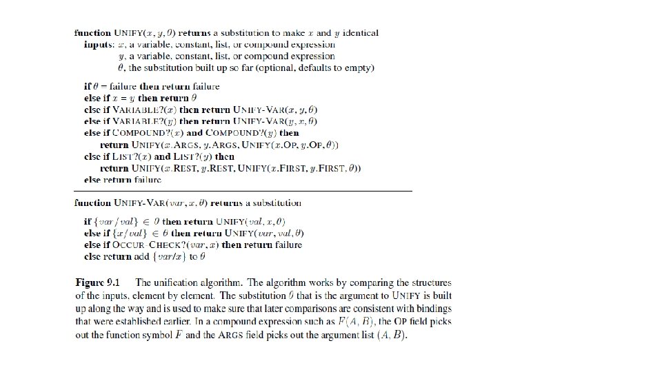
• The UNIFY algorithm takes two sentences and returns a unifier for them if one exists: UNIFY(p, q)=θ where SUBST(θ, p)= SUBST(θ, q). • Suppose we have a query Ask. Vars(Knows(John, x)): whom does John know? Answers to this query can be found by finding all sentences in the knowledge base that unify with Knows(John, x). • Here are the results of unification with four different sentences that might be in the knowledge base: • The last unification fails because x cannot take on the values John and Elizabeth at the same time. • Now, remember that Knows(x, Elizabeth) means “Everyone knows Elizabeth, ” so we should be able to infer that John knows Elizabeth. • The problem arises only because the two sentences happen to use the same variable name, x. • The problem can be avoided by standardizing apart one of the two sentences being unified, which means renaming its variables to avoid name clashes. • For example, we can rename x in Knows(x, Elizabeth) to x 17 (a new variable name) without changing its meaning. Now the unification will work:

• There is one more complication: we said that UNIFY should return a substitution that makes the two arguments look the same. But there could be more than one such unifier. • For example, UNIFY(Knows(John, x), Knows(y, z)) could return {y/John, x/z} or {y/John, x/John, z/John}. • The first unifier gives Knows(John, z) as the result of unification, whereas the second gives Knows(John, John). • The second result could be obtained from the first by an additional substitution {z/John}; we say that the first unifier is more general than the second, because it places fewer restrictions on the values of the variables. • It turns out that, for every unifiable pair of expressions, there is a single most general unifier (or MGU) that is unique up to renaming and substitution of variables. • (For example, {x/John} and {y/John} are considered equivalent, as are {x/John, y/John} and {x/John, y/x}. ) In this case it is {y/John, x/z}. • The process is simple: recursively explore the two expressions simultaneously “side by side, ” building up a unifier along the way, but failing if two corresponding points in the structures do not match. • There is one expensive step: when matching a variable against a complex term, one must check whether the variable itself occurs inside the term; if it does, the match fails because no consistent unifier can be constructed. • For example, S(x) can’t unify with S(S(x)). This so called occur check makes the complexity of the entire algorithm quadratic in the size of the expressions being unified.

Storage and retrieval • Underlying the TELL and ASK functions used to inform and interrogate a knowledge base are the more primitive STORE and FETCH functions. • STORE(s) stores a sentence s into the knowledge base and FETCH(q) returns all unifiers such that the query q unifies with some sentence in the knowledge base. • The problem we used to illustrate unification—finding all facts that unify with Knows(John, x)—is an instance of FETCHing. • The simplest way to implement STORE and FETCH is to keep all the facts in one long list and unify each query against every element of the list. • We can make FETCH more efficient by ensuring that unifications are attempted only with sentences that have some chance of unifying. • For example, there is no point in trying to unify Knows(John, x) with Brother (Richard, John). • We can avoid such unifications by indexing the facts in the knowledge base. • A simple scheme called predicate indexing puts all the Knows facts in one bucket and all the Brother facts in another. • The buckets can be stored in a hash table for efficient access.

• Predicate indexing is useful when there are many predicate symbols but only a few clauses for each symbol. Sometimes, however, a predicate has many clauses. • For example, suppose that the tax authorities want to keep track of who employs whom, using a predicate Employs(x, y). • This would be a very large bucket with perhaps millions of employers and tens of millions of employees. • Answering a query such as Employs(x, Richard) with predicate indexing would require scanning the entire bucket. • For this particular query, it would help if facts were indexed both by predicate and by second argument, perhaps using a combined hash table key. • Then we could simply construct the key from the query and retrieve exactly those facts that unify with the query.

• For other queries, such as Employs(IBM, y), we would need to have indexed the facts by combining the predicate with the first argument. • Therefore, facts can be stored under multiple index keys, rendering them instantly accessible to various queries that they might unify with. • Given a sentence to be stored, it is possible to construct indices for all possible queries that unify with it. For the fact Employs(IBM, Richard), the queries are Employs(IBM, Richard) Does IBM employ Richard? Employs(x, Richard) Who employs Richard? Employs(IBM, y) Whom does IBM employ? Employs(x, y) Who employs whom? • These queries form a subsumption lattice, as shown in Figure 9. 2(a). • The lattice has some interesting properties. • For example, the child of any node in the lattice is obtained from its parent by a single substitution; and the “highest” common descendant of any two nodes is the result of applying their most general unifier. • A sentence with repeated constants has a slightly different lattice, as shown in Figure 9. 2(b). • Function symbols and variables in the sentences to be stored introduce still more interesting lattice structures.

FORWARD CHAINING • The idea is simple: start with the atomic sentences in the knowledge base and apply Modus Ponens in the forward direction, adding new atomic sentences, until no further inferences can be made. • Here, we explain how the algorithm is applied to first-order definite clauses. • Definite clauses such as Situation ⇒ Response are especially useful for systems that make inferences in response to newly arrived information. • Many systems can be defined this way, and forward chaining can be implemented very efficiently. First-order definite clauses • First-order definite clauses closely resemble propositional definite clauses - they are disjunctions of literals of which exactly one is positive. • A definite clause either is atomic or is an implication whose antecedent is a conjunction of positive literals and whose consequent is a single positive literal. The following are first-order definite clauses: King(x) ^ Greedy(x) ⇒ Evil(x). King(John). Greedy(y). • Unlike propositional literals, first-order literals can include variables, in which case those variables are assumed to be universally quantified.

• Consider the following problem: • The law says that it is a crime for an American to sell weapons to hostile nations. The country Nono, an enemy of America, has some missiles, and all of its missiles were sold to it by Colonel West, who is American. • We will prove that West is a criminal. First, we will represent these facts as first-order definite clauses. • The next section shows how the forward-chaining algorithm solves the problem. • “. . . it is a crime for an American to sell weapons to hostile nations”: American(x) ^Weapon(y) ^ Sells(x, y, z) ^ Hostile(z) ⇒ Criminal (x). (9. 3) • “Nono. . . has some missiles. ” The sentence ∃ x Owns(Nono, x)^Missile(x) is transformed into two definite clauses by Existential Instantiation, introducing a new constant M 1: Owns(Nono, M 1) (9. 4) Missile(M 1) (9. 5) • “All of its missiles were sold to it by Colonel West”: Missile(x) ^ Owns(Nono, x) ⇒ Sells(West , x, Nono). (9. 6) • We will also need to know that missiles are weapons: Missile(x) ⇒ Weapon(x) (9. 7)

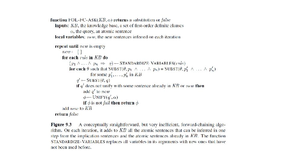
• and we must know that an enemy of America counts as “hostile”: Enemy(x, America) ⇒ Hostile(x). (9. 8) • “West, who is American. . . ”: American(West). (9. 9) • “The country Nono, an enemy of America. . . ”: Enemy(Nono, America). (9. 10) • This knowledge base contains no function symbols and is therefore an instance of the class of Datalog knowledge bases. • Datalog is a language that is restricted to first-order definite clauses with no function symbols. • Datalog gets its name because it can represent the type of statements typically made in relational databases. A simple forward-chaining algorithm • The first forward-chaining algorithm we consider is a simple one, shown in Figure 9. 3. Starting from the known facts, it triggers all the rules whose premises are satisfied, adding their conclusions to the known facts. • The process repeats until the query is answered (assuming that just one answer is required) or no new facts are added. Notice that a fact is not “new” if it is just a renaming of a known fact.

• One sentence is a renaming of another if they are identical except for the names of the variables. • For example, Likes(x, Ice. Cream) and Likes(y, Ice. Cream) are renamings of each other because they differ only in the choice of x or y; their meanings are identical: everyone likes ice cream. • We use our crime problem to illustrate how FOL-FC-ASK works. The implication sentences are (9. 3), (9. 6), (9. 7), and (9. 8). Two iterations are required:

• Figure 9. 4 shows the proof tree that is generated. • Notice that no new inferences are possible at this point because every sentence that could be concluded by forward chaining is already contained explicitly in the KB. • Such a knowledge base is called a fixed point of the inference process. • Fixed points reached by forward chaining with first-order definite clauses are similar to those for propositional forward chaining. • The principal difference is that a first order fixed point can include universally quantified atomic sentences.

• FOL-FC-ASK is easy to analyze. First, it is sound, because every inference is just an application of Generalized Modus Ponens, which is sound. • Second, it is complete for definite clause knowledge bases; that is, it answers every query whose answers are entailed by any knowledge base of definite clauses. • For Datalog knowledge bases, which contain no function symbols, the proof of completeness is fairly easy. • We begin by counting the number of possible facts that can be added, which determines the maximum number of iterations. • Let k be the maximum arity (number of arguments) of any predicate, p be the number of predicates, and n be the number of constant symbols. Clearly, there can be no more than pnk distinct ground facts, so after this many iterations the algorithm must have reached a fixed point. • Then we can make an argument very similar to the proof of completeness for propositional forward chaining. • The details of how to make the transition from propositional to first-order completeness are given for the resolution algorithm.

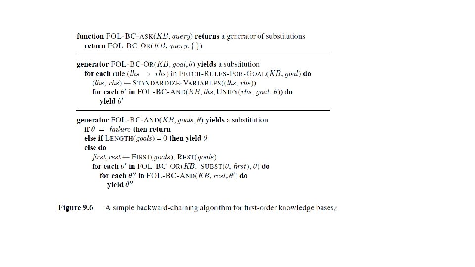
BACKWARD CHAINING • This algorithm works backward from the goal, chaining through rules to find known facts that support the proof. • Figure 9. 6 shows a backward-chaining algorithm for definite clauses. • FOL-BC-ASK(KB, goal ) will be proved if the knowledge base contains a clause of the form lhs ) goal , where lhs (left-hand side) is a list of conjuncts. • An atomic fact like American(West) is considered as a clause whose lhs is the empty list. • Now a query that contains variables might be proved in multiple ways. • For example, the query Person(x) could be proved with the substitution {x/John} as well as with {x/Richard}. So we implement FOL- BC-ASK as a generator— a function that returns multiple times, each time giving one possible result. • Backward chaining is a kind of AND/OR search—the OR part because the goal query can be proved by any rule in the knowledge base, and the AND part because all the conjuncts in the lhs of a clause must be proved. • FOL-BC-OR works by fetching all clauses that might unify with the goal, standardizing the variables in the clause to be brand-new variables, and then, if the rhs of the clause does indeed unify with the goal, proving every conjunct in the lhs, using FOL-BC-AND.

• • Figure 9. 7 is the proof tree for deriving Criminal (West) from sentences (9. 3) through (9. 10). Backward chaining, as we have written it, is clearly a depth-first search algorithm. This means that its space requirements are linear in the size of the proof. It also means that backward chaining (unlike forward chaining) suffers from problems with repeated states and incompleteness.