Indexing and Execution May 20 th 2002 Indexing

Indexing and Execution May 20 th, 2002

Indexing - Recap • Primary file organization: heap, sorted, hashed. • Primary vs. secondary • Clustered vs. unclustered • Dense vs. sparse • Composite search key indexes. • Not all combinations are possible. • Next: B+-trees.

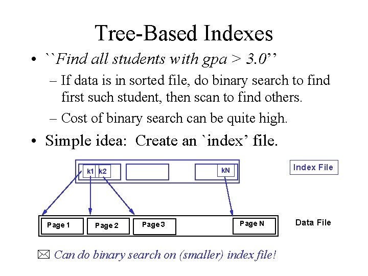
Tree-Based Indexes • ``Find all students with gpa > 3. 0’’ – If data is in sorted file, do binary search to find first such student, then scan to find others. – Cost of binary search can be quite high. • Simple idea: Create an `index’ file. Page 1 Page 2 Index File k. N k 1 k 2 Page 3 Page N * Can do binary search on (smaller) index file! Data File

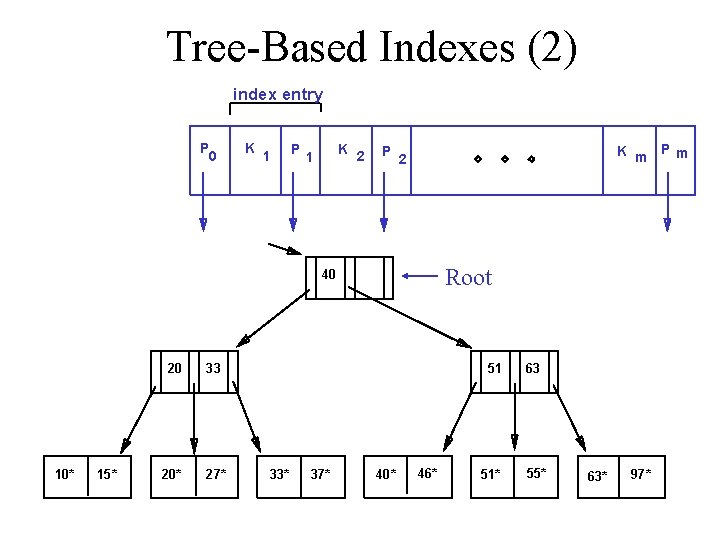
Tree-Based Indexes (2) index entry P 0 K 1 P K 2 1 P K m 2 Root 40 10* 15* 20 33 20* 27* 51 33* 37* 40* 46* 51* 63 55* 63* 97* Pm

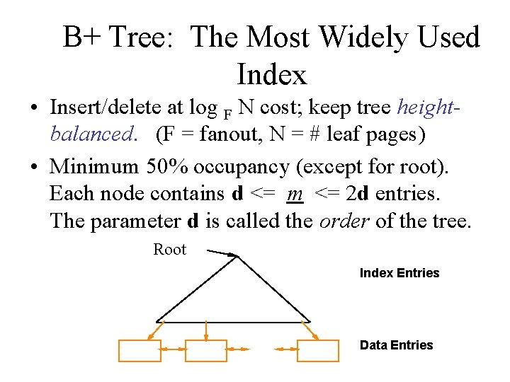
B+ Tree: The Most Widely Used Index • Insert/delete at log F N cost; keep tree heightbalanced. (F = fanout, N = # leaf pages) • Minimum 50% occupancy (except for root). Each node contains d <= m <= 2 d entries. The parameter d is called the order of the tree. Root Index Entries Data Entries

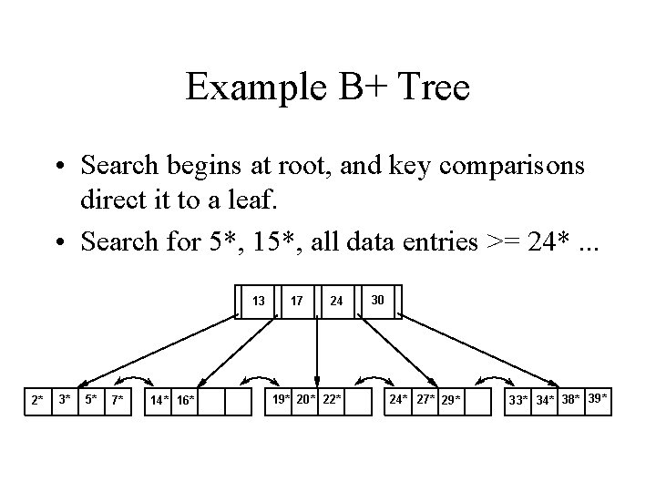
Example B+ Tree • Search begins at root, and key comparisons direct it to a leaf. • Search for 5*, 15*, all data entries >= 24*. . . 13 2* 3* 5* 7* 14* 16* 17 24 19* 20* 22* 30 24* 27* 29* 33* 34* 38* 39*

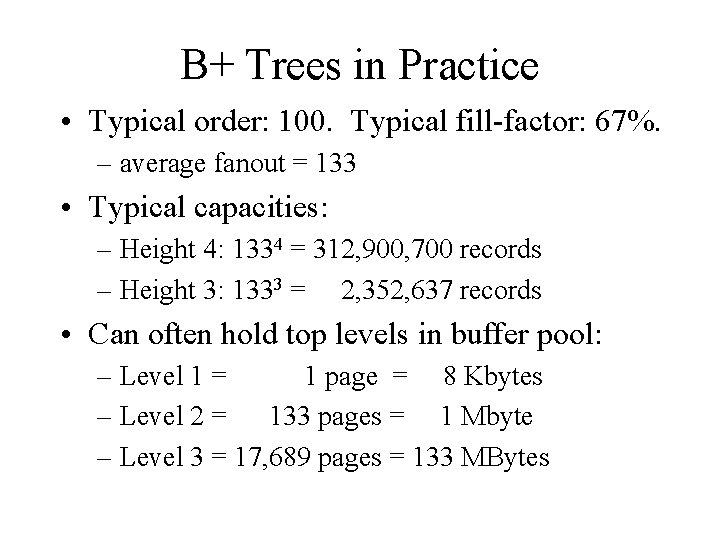
B+ Trees in Practice • Typical order: 100. Typical fill-factor: 67%. – average fanout = 133 • Typical capacities: – Height 4: 1334 = 312, 900, 700 records – Height 3: 1333 = 2, 352, 637 records • Can often hold top levels in buffer pool: – Level 1 = 1 page = 8 Kbytes – Level 2 = 133 pages = 1 Mbyte – Level 3 = 17, 689 pages = 133 MBytes

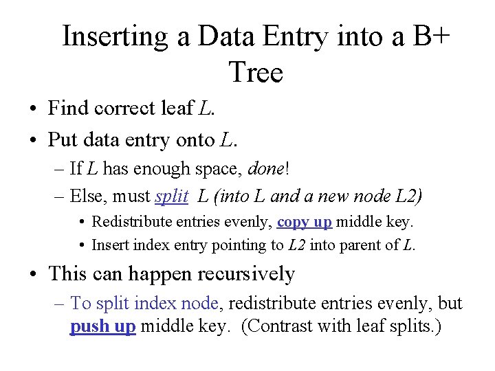
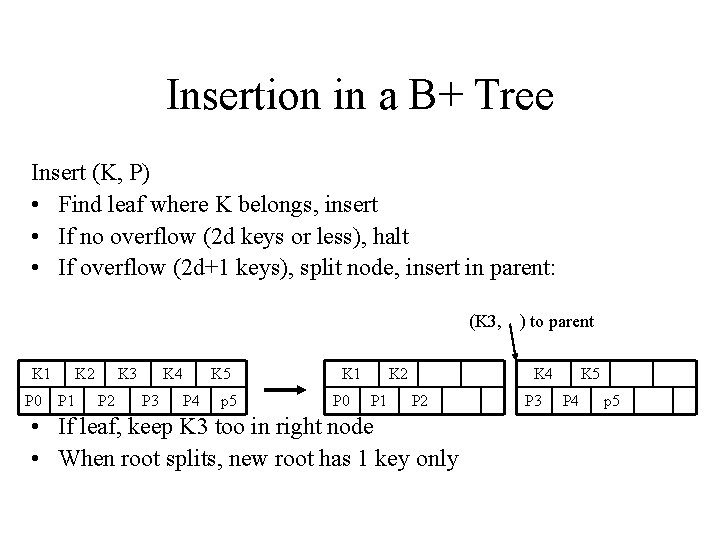
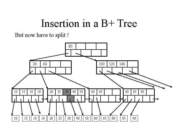
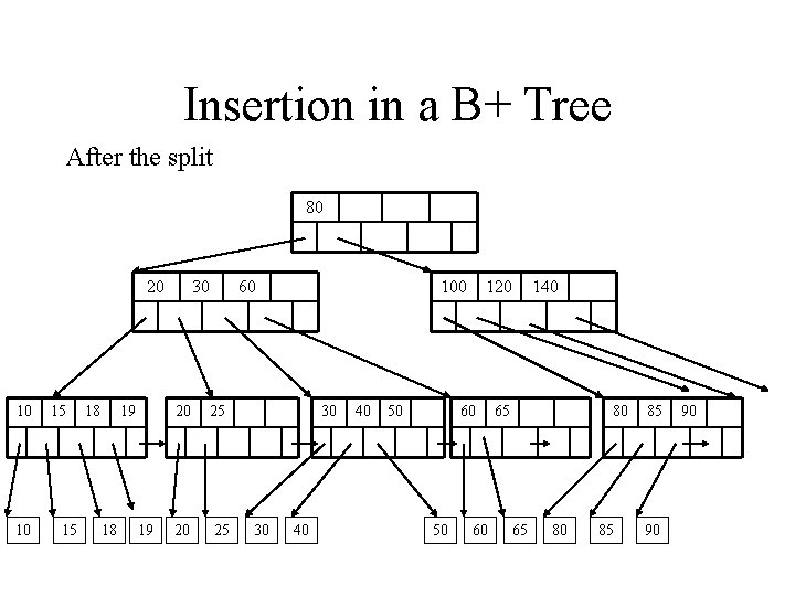
Inserting a Data Entry into a B+ Tree • Find correct leaf L. • Put data entry onto L. – If L has enough space, done! – Else, must split L (into L and a new node L 2) • Redistribute entries evenly, copy up middle key. • Insert index entry pointing to L 2 into parent of L. • This can happen recursively – To split index node, redistribute entries evenly, but push up middle key. (Contrast with leaf splits. )

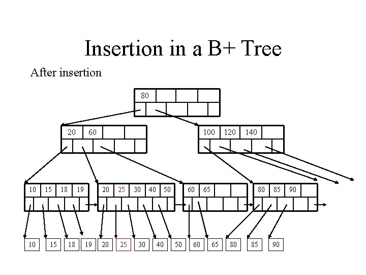
Insertion in a B+ Tree Insert (K, P) • Find leaf where K belongs, insert • If no overflow (2 d keys or less), halt • If overflow (2 d+1 keys), split node, insert in parent: (K 3, K 1 P 0 K 2 P 1 K 3 P 2 K 4 P 3 P 4 K 5 p 5 K 1 P 0 K 2 P 1 ) to parent K 4 P 2 • If leaf, keep K 3 too in right node • When root splits, new root has 1 key only P 3 K 5 P 4 p 5

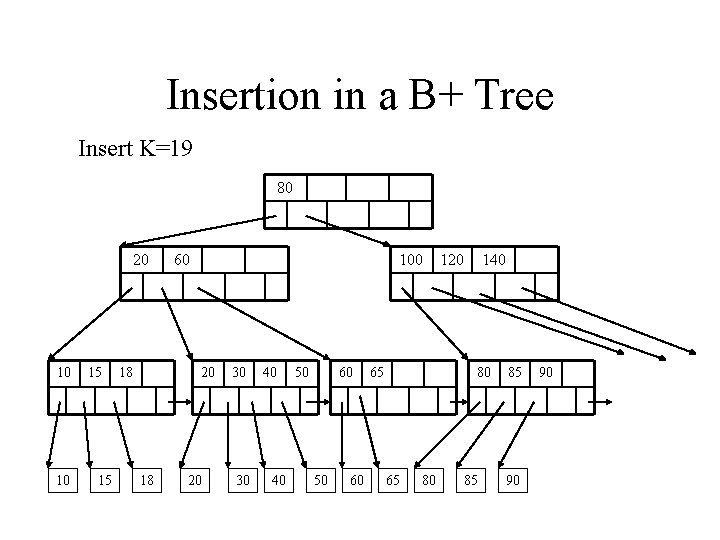
Insertion in a B+ Tree Insert K=19 80 20 10 10 15 15 18 60 100 20 18 20 30 30 40 40 50 60 65 120 140 80 65 80 85 85 90 90

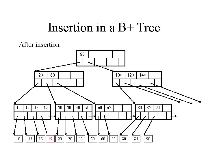
Insertion in a B+ Tree After insertion 80 20 10 10 15 15 18 60 19 18 19 100 20 30 40 40 50 60 65 120 140 80 65 80 85 85 90 90

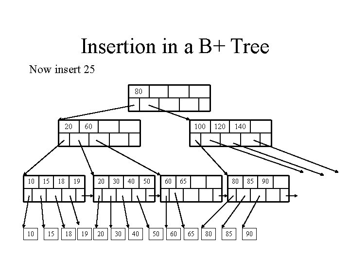
Insertion in a B+ Tree Now insert 25 80 20 10 10 15 15 18 60 19 18 19 100 20 30 40 40 50 60 65 120 140 80 65 80 85 85 90 90

Insertion in a B+ Tree After insertion 80 20 10 10 15 15 18 60 19 18 19 100 20 25 30 30 40 50 40 60 50 60 120 65 140 80 65 80 85 85 90 90

Insertion in a B+ Tree But now have to split ! 80 20 10 10 15 15 18 60 19 18 19 100 20 25 30 30 40 50 40 60 50 60 120 65 140 80 65 80 85 85 90 90

Insertion in a B+ Tree After the split 80 20 10 10 15 15 18 19 30 60 20 25 100 30 30 40 40 50 120 60 50 60 140 65 80 85 85 90 90

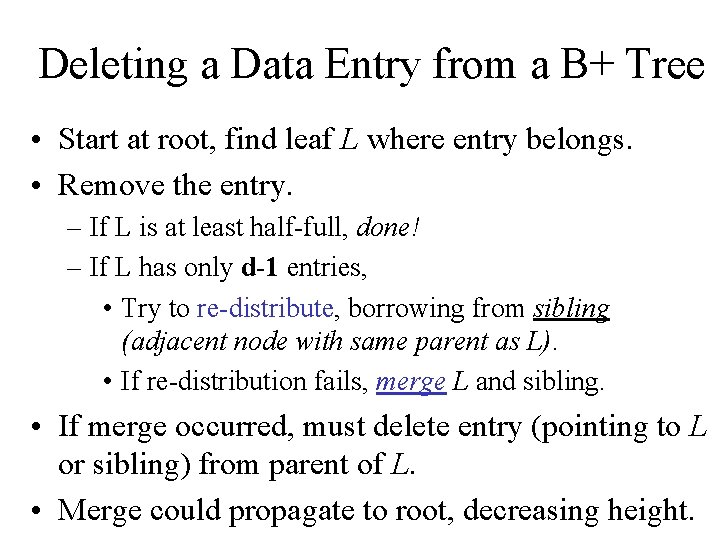
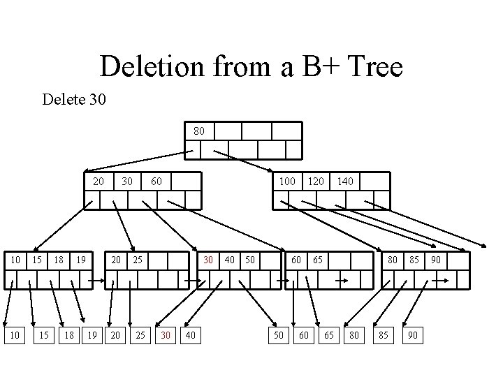
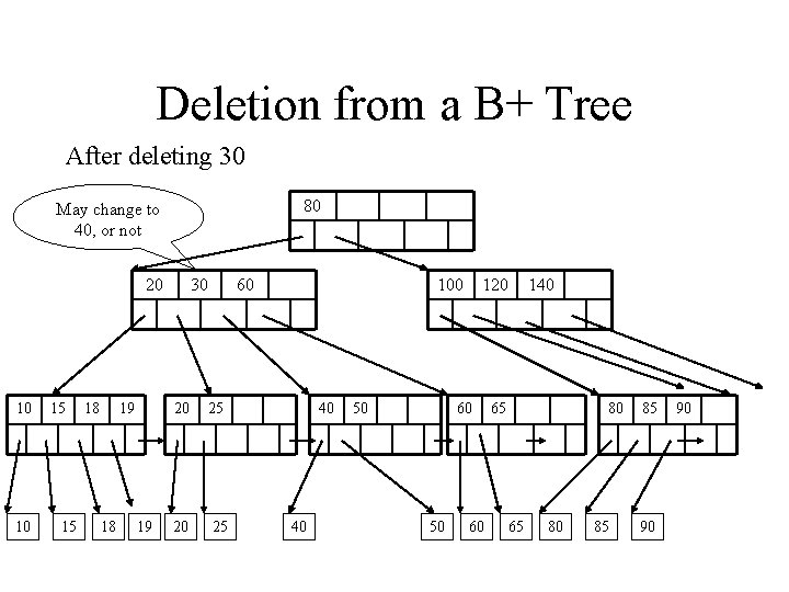
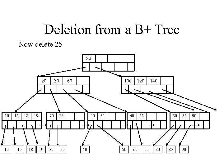
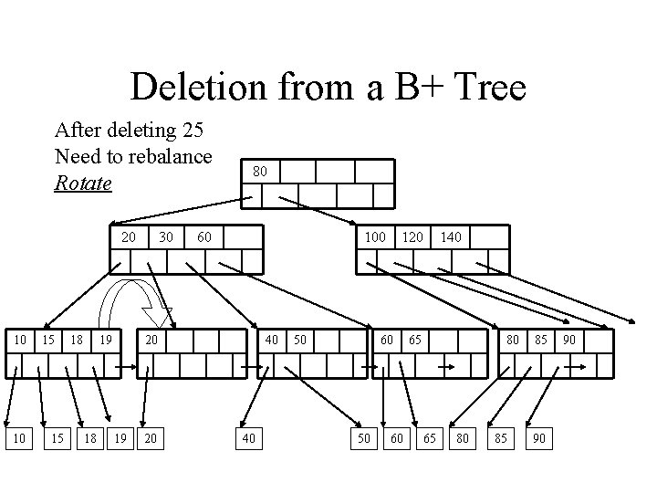
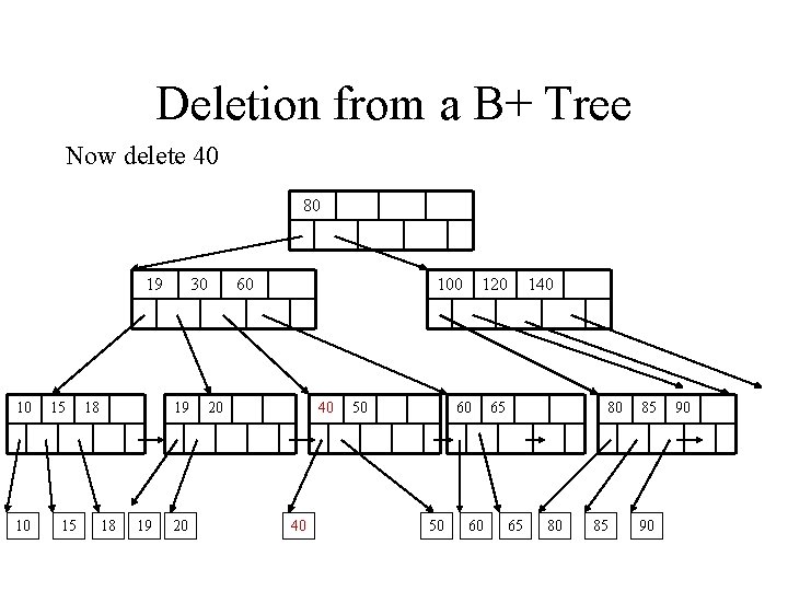
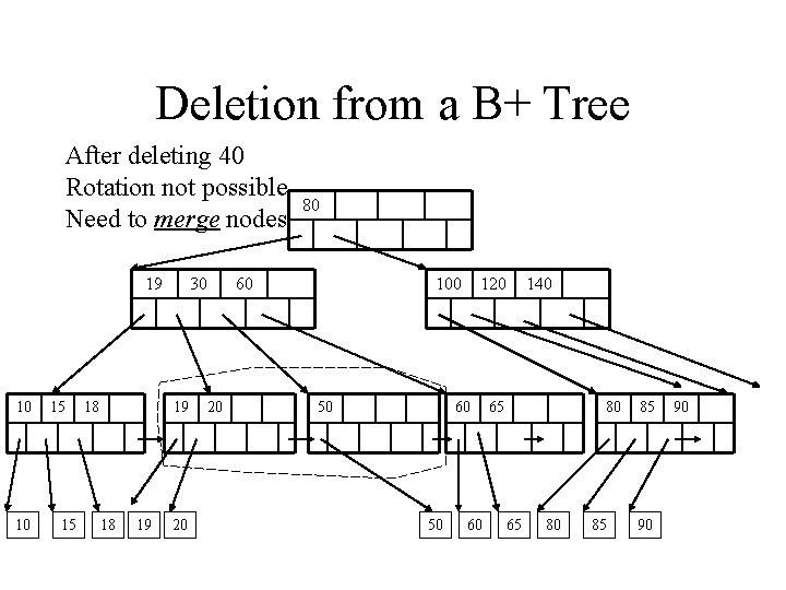
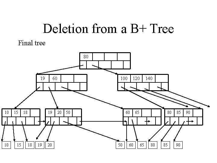
Deleting a Data Entry from a B+ Tree • Start at root, find leaf L where entry belongs. • Remove the entry. – If L is at least half-full, done! – If L has only d-1 entries, • Try to re-distribute, borrowing from sibling (adjacent node with same parent as L). • If re-distribution fails, merge L and sibling. • If merge occurred, must delete entry (pointing to L or sibling) from parent of L. • Merge could propagate to root, decreasing height.

Deletion from a B+ Tree Delete 30 80 20 10 10 15 15 18 19 30 60 20 25 100 30 30 40 40 50 120 60 50 60 140 65 80 85 85 90 90

Deletion from a B+ Tree After deleting 30 80 May change to 40, or not 20 10 10 15 15 18 19 30 60 20 25 100 40 40 50 120 60 50 60 140 65 80 85 85 90 90

Deletion from a B+ Tree Now delete 25 80 20 10 10 15 15 18 19 30 60 20 25 100 40 40 50 120 60 50 60 140 65 80 85 85 90 90

Deletion from a B+ Tree After deleting 25 Need to rebalance Rotate 20 10 10 15 15 18 19 18 30 80 60 100 20 19 20 40 40 50 120 60 50 60 140 65 80 85 85 90 90

Deletion from a B+ Tree Now delete 40 80 19 10 10 15 15 18 30 19 18 19 20 60 100 20 40 40 50 120 60 50 60 140 65 80 85 85 90 90

Deletion from a B+ Tree After deleting 40 Rotation not possible Need to merge nodes 19 10 10 15 15 18 30 19 18 19 20 20 80 60 100 50 120 60 50 60 140 65 80 85 85 90 90

Deletion from a B+ Tree Final tree 80 19 10 10 15 15 18 60 19 18 19 20 20 100 50 120 60 50 60 140 65 80 85 85 90 90

Issues in Indexing • Multi-dimensional indexing: – how do we index regions in space? – Document collections? – Multi-dimensional sales data – How do we support nearest neighbor queries? • Indexing is still a hot and unsolved problem!

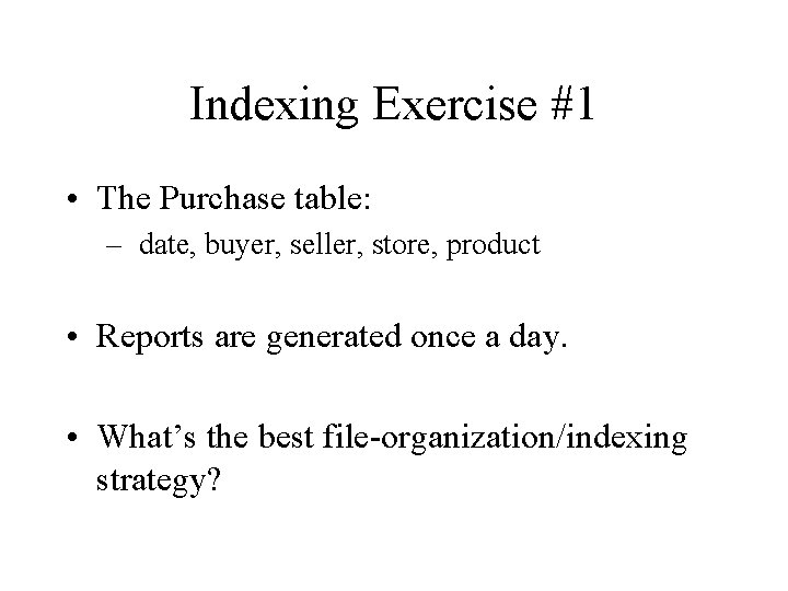
Indexing Exercise #1 • The Purchase table: – date, buyer, seller, store, product • Reports are generated once a day. • What’s the best file-organization/indexing strategy?

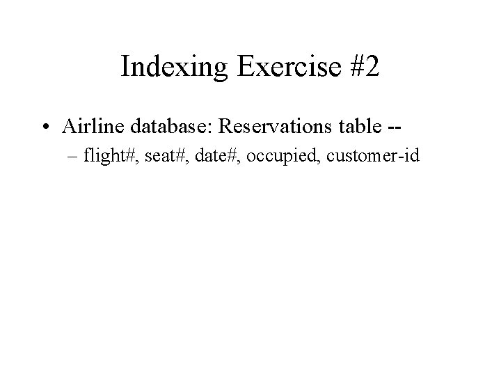
Indexing Exercise #2 • Airline database: Reservations table -– flight#, seat#, date#, occupied, customer-id

Indexing Exercise #3 • Web log application: load all the logs every night into a database. • Generate reports every day (for curious professors).

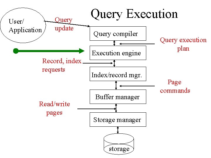
User/ Application Query update Query Execution Query compiler Execution engine Record, index requests Read/write pages Index/record mgr. Buffer manager Storage manager storage Query execution plan Page commands

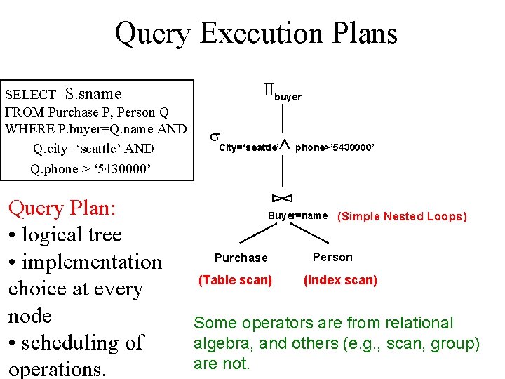
Query Execution Plans SELECT S. sname FROM Purchase P, Person Q WHERE P. buyer=Q. name AND Q. city=‘seattle’ AND Q. phone > ‘ 5430000’ Query Plan: • logical tree • implementation choice at every node • scheduling of operations. buyer City=‘seattle’ phone>’ 5430000’ Buyer=name Purchase (Table scan) (Simple Nested Loops) Person (Index scan) Some operators are from relational algebra, and others (e. g. , scan, group) are not.

The Leaves of the Plan: Scans • Table scan: iterate through the records of the relation. • Index scan: go to the index, from there get the records in the file (when would this be better? ) • Sorted scan: produce the relation in order. Implementation depends on relation size.

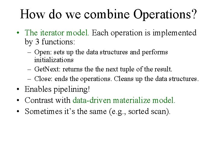
How do we combine Operations? • The iterator model. Each operation is implemented by 3 functions: – Open: sets up the data structures and performs initializations – Get. Next: returns the next tuple of the result. – Close: ends the operations. Cleans up the data structures. • Enables pipelining! • Contrast with data-driven materialize model. • Sometimes it’s the same (e. g. , sorted scan).

Implementing Relational Operations • We will consider how to implement: – Selection ( ) Selects a subset of rows from relation. – Projection ( ) Deletes unwanted columns from relation. – Join ( ) Allows us to combine two relations. – Set-difference Tuples in reln. 1, but not in reln. 2. – Union Tuples in reln. 1 and in reln. 2. – Aggregation (SUM, MIN, etc. ) and GROUP BY

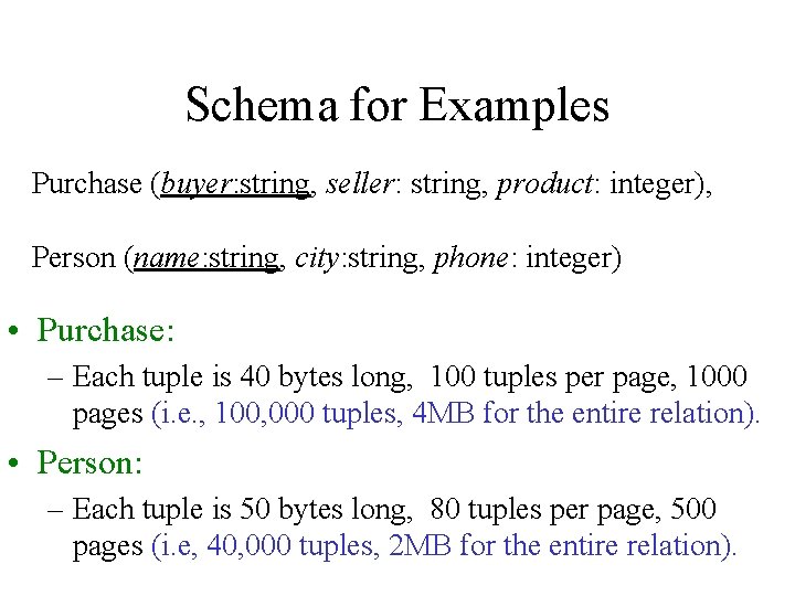
Schema for Examples Purchase (buyer: string, seller: string, product: integer), Person (name: string, city: string, phone: integer) • Purchase: – Each tuple is 40 bytes long, 100 tuples per page, 1000 pages (i. e. , 100, 000 tuples, 4 MB for the entire relation). • Person: – Each tuple is 50 bytes long, 80 tuples per page, 500 pages (i. e, 40, 000 tuples, 2 MB for the entire relation).

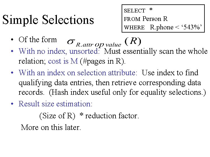
Simple Selections SELECT * FROM Person R WHERE R. phone < ‘ 543%’ • Of the form • With no index, unsorted: Must essentially scan the whole relation; cost is M (#pages in R). • With an index on selection attribute: Use index to find qualifying data entries, then retrieve corresponding data records. (Hash index useful only for equality selections. ) • Result size estimation: (Size of R) * reduction factor. More on this later.

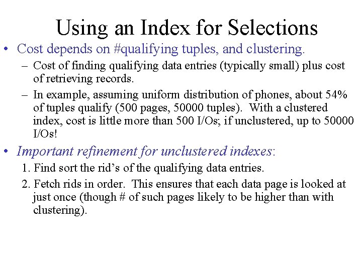
Using an Index for Selections • Cost depends on #qualifying tuples, and clustering. – Cost of finding qualifying data entries (typically small) plus cost of retrieving records. – In example, assuming uniform distribution of phones, about 54% of tuples qualify (500 pages, 50000 tuples). With a clustered index, cost is little more than 500 I/Os; if unclustered, up to 50000 I/Os! • Important refinement for unclustered indexes: 1. Find sort the rid’s of the qualifying data entries. 2. Fetch rids in order. This ensures that each data page is looked at just once (though # of such pages likely to be higher than with clustering).

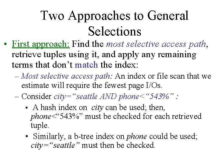
Two Approaches to General Selections • First approach: Find the most selective access path, retrieve tuples using it, and apply any remaining terms that don’t match the index: – Most selective access path: An index or file scan that we estimate will require the fewest page I/Os. – Consider city=“seattle AND phone<“ 543%” : • A hash index on city can be used; then, phone<“ 543%” must be checked for each retrieved tuple. • Similarly, a b-tree index on phone could be used; city=“seattle” must then be checked.

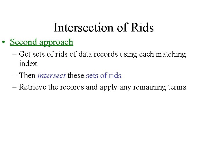
Intersection of Rids • Second approach – Get sets of rids of data records using each matching index. – Then intersect these sets of rids. – Retrieve the records and apply any remaining terms.

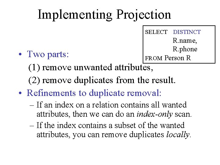
Implementing Projection SELECT DISTINCT R. name, R. phone FROM Person R • Two parts: (1) remove unwanted attributes, (2) remove duplicates from the result. • Refinements to duplicate removal: – If an index on a relation contains all wanted attributes, then we can do an index-only scan. – If the index contains a subset of the wanted attributes, you can remove duplicates locally.

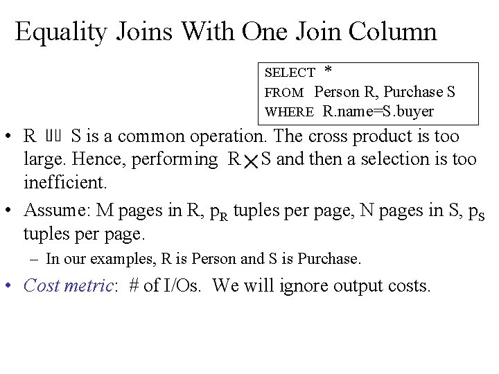
Equality Joins With One Join Column SELECT * FROM Person R, Purchase WHERE R. name=S. buyer S • R S is a common operation. The cross product is too large. Hence, performing R S and then a selection is too inefficient. • Assume: M pages in R, p. R tuples per page, N pages in S, p. S tuples per page. – In our examples, R is Person and S is Purchase. • Cost metric: # of I/Os. We will ignore output costs.

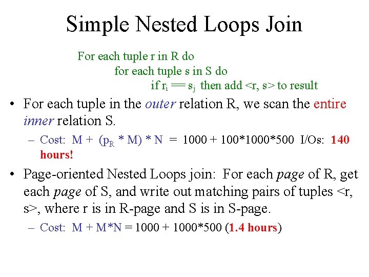
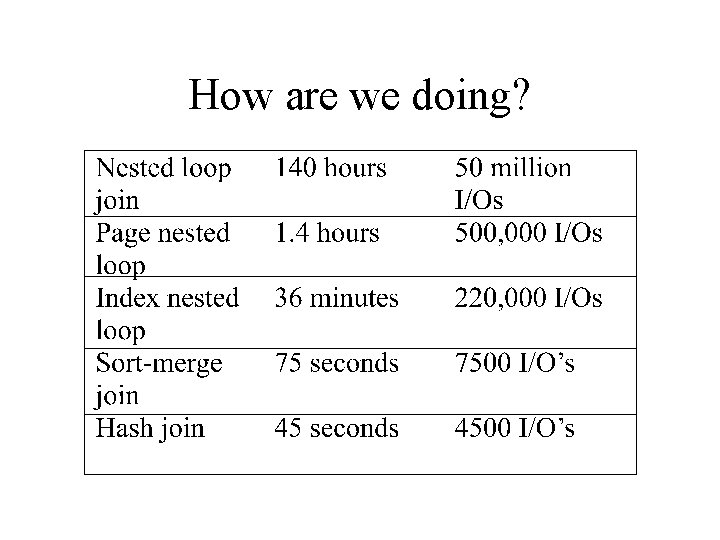
Simple Nested Loops Join For each tuple r in R do for each tuple s in S do if ri == sj then add <r, s> to result • For each tuple in the outer relation R, we scan the entire inner relation S. – Cost: M + (p. R * M) * N = 1000 + 100*1000*500 I/Os: 140 hours! • Page-oriented Nested Loops join: For each page of R, get each page of S, and write out matching pairs of tuples <r, s>, where r is in R-page and S is in S-page. – Cost: M + M*N = 1000 + 1000*500 (1. 4 hours)

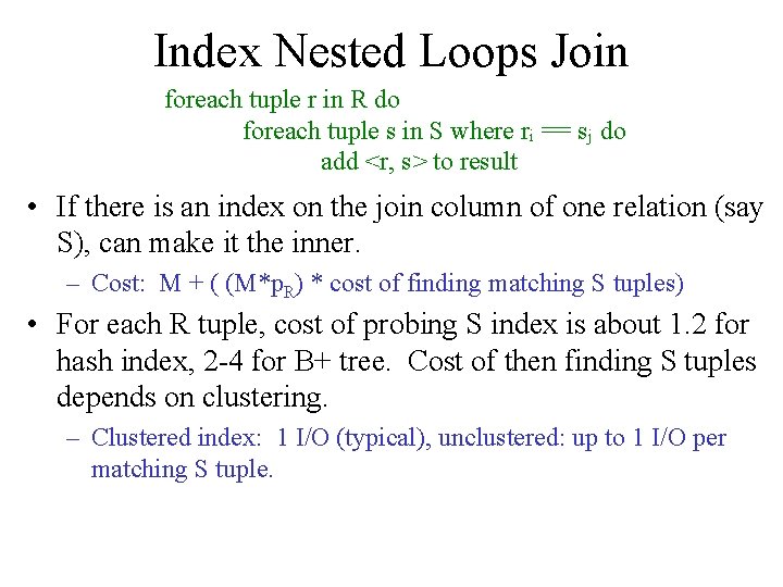
Index Nested Loops Join foreach tuple r in R do foreach tuple s in S where ri == sj do add <r, s> to result • If there is an index on the join column of one relation (say S), can make it the inner. – Cost: M + ( (M*p. R) * cost of finding matching S tuples) • For each R tuple, cost of probing S index is about 1. 2 for hash index, 2 -4 for B+ tree. Cost of then finding S tuples depends on clustering. – Clustered index: 1 I/O (typical), unclustered: up to 1 I/O per matching S tuple.

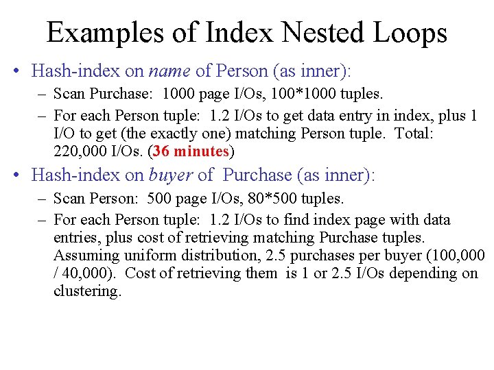
Examples of Index Nested Loops • Hash-index on name of Person (as inner): – Scan Purchase: 1000 page I/Os, 100*1000 tuples. – For each Person tuple: 1. 2 I/Os to get data entry in index, plus 1 I/O to get (the exactly one) matching Person tuple. Total: 220, 000 I/Os. (36 minutes) • Hash-index on buyer of Purchase (as inner): – Scan Person: 500 page I/Os, 80*500 tuples. – For each Person tuple: 1. 2 I/Os to find index page with data entries, plus cost of retrieving matching Purchase tuples. Assuming uniform distribution, 2. 5 purchases per buyer (100, 000 / 40, 000). Cost of retrieving them is 1 or 2. 5 I/Os depending on clustering.

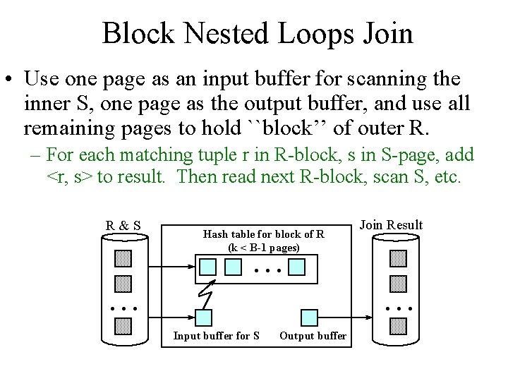
Block Nested Loops Join • Use one page as an input buffer for scanning the inner S, one page as the output buffer, and use all remaining pages to hold ``block’’ of outer R. – For each matching tuple r in R-block, s in S-page, add <r, s> to result. Then read next R-block, scan S, etc. R&S Hash table for block of R (k < B-1 pages) Join Result . . Input buffer for S Output buffer

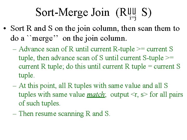
Sort-Merge Join (R i=j S) • Sort R and S on the join column, then scan them to do a ``merge’’ on the join column. – Advance scan of R until current R-tuple >= current S tuple, then advance scan of S until current S-tuple >= current R tuple; do this until current R tuple = current S tuple. – At this point, all R tuples with same value and all S tuples with same value match; output <r, s> for all pairs of such tuples. – Then resume scanning R and S.

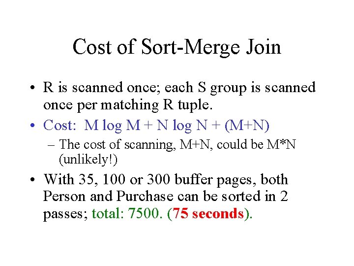
Cost of Sort-Merge Join • R is scanned once; each S group is scanned once per matching R tuple. • Cost: M log M + N log N + (M+N) – The cost of scanning, M+N, could be M*N (unlikely!) • With 35, 100 or 300 buffer pages, both Person and Purchase can be sorted in 2 passes; total: 7500. (75 seconds).

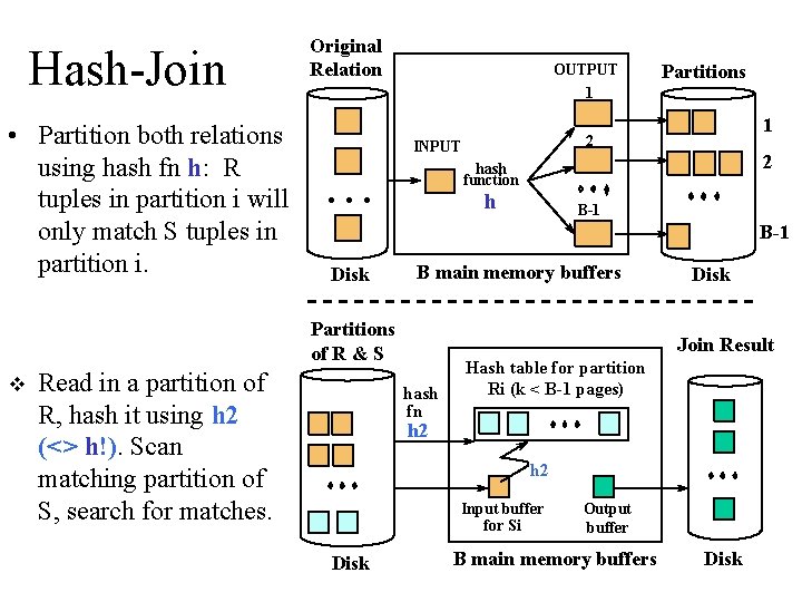
Hash-Join • Partition both relations using hash fn h: R tuples in partition i will only match S tuples in partition i. Original Relation OUTPUT 1 1 2 INPUT 2 hash function . . . h B-1 Disk B main memory buffers Partitions of R & S v Partitions Read in a partition of R, hash it using h 2 (<> h!). Scan matching partition of S, search for matches. Disk Join Result hash fn Hash table for partition Ri (k < B-1 pages) h 2 Input buffer for Si Disk Output buffer B main memory buffers Disk

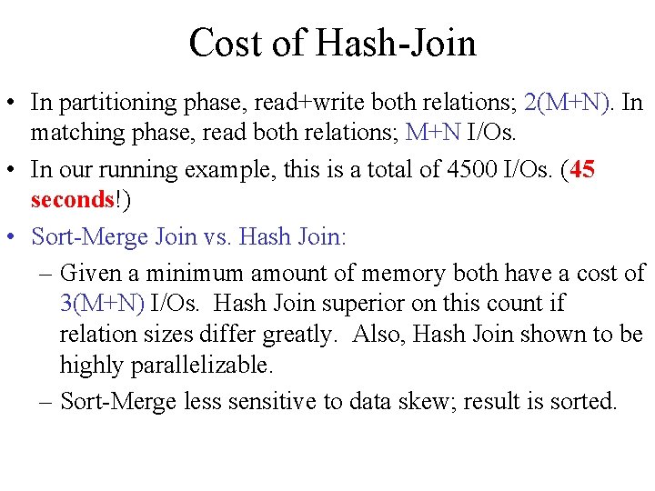
Cost of Hash-Join • In partitioning phase, read+write both relations; 2(M+N). In matching phase, read both relations; M+N I/Os. • In our running example, this is a total of 4500 I/Os. (45 seconds!) • Sort-Merge Join vs. Hash Join: – Given a minimum amount of memory both have a cost of 3(M+N) I/Os. Hash Join superior on this count if relation sizes differ greatly. Also, Hash Join shown to be highly parallelizable. – Sort-Merge less sensitive to data skew; result is sorted.

How are we doing?

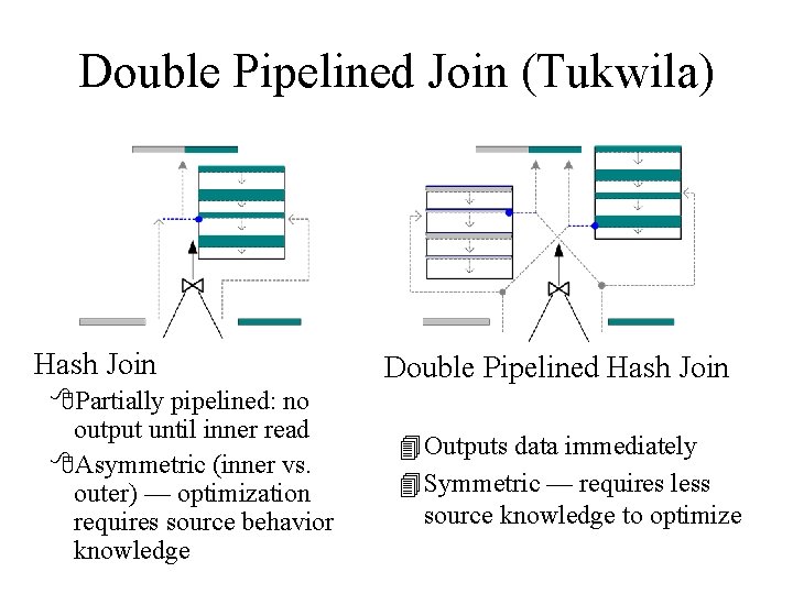
Double Pipelined Join (Tukwila) Hash Join 8 Partially pipelined: no output until inner read 8 Asymmetric (inner vs. outer) — optimization requires source behavior knowledge Double Pipelined Hash Join 4 Outputs data immediately 4 Symmetric — requires less source knowledge to optimize