High sensitivity wavefront sensing with the nonlinear curvature

High sensitivity wavefront sensing with the non-linear curvature WFS Olivier Guyon University of Arizona Subaru Telescope Mala Mateen Starfire Optical Range University of Arizona 1

Some fundamental desirable WFS properties Linearity: The WFS response should be a linear function of the input phase - simplifies control algorithm - minimizes computation time -> important for fast systems Capture range: The WFS should be able to measure large WF errors - the loop can be closed on natural seeing - possible to use the WFS in open loop - possible to “dial in” large offset aberrations Sensitivity: The WFS should make efficient use of the incoming photons - the AO system can then maintain high performance on fainter sources - the AO system can run faster I will show in the next slides that it is not possible to get all 3 properties simultaneously, and the WFS needs to be carefully chosen to fit the AO system requirements.

Wavefront Sensor Options. . . Linearity, dynamical range and sensitivity Linear, large dynamical range, poor sensitivity: Shack-Hartmann (SH) Curvature (Curv) Modulated Pyramid (MPyr) Linear, small dynamical range, high sensitivity: Fixed Pyramid (FPyr) Zernike phase constrast mask (ZPM) Pupil plane Mach-Zehnder interferometer (PPMZ) Non-linear, moderate to large dynamical range, high sensitivity: Non-linear Curvature (nl. Curv) Non-linear Pyramid (nl. Pyr) ?

High sensitivity WFS : Three examples ● ● ● Fixed Pyramid WFS: A pyramid is placed in the focal plane. The starlight hits the tip of the pyramid Zernike phase contrast: A small phase shifting mask is placed in the focal plane. Roughly 1/2 of the light goes through, 1/2 goes around. The two halves interfere to give an intensity signal Mach-Zehnder / Self-referencing interferometer / point diffraction interferometer: An interferometer is assembled by splitting the beam in 2 and recombining the two halves. On one of the arms, a spatial filter (pinhole) is placed to create the “reference” beam which interferes with the wavefront These 3 options are Linear but will fail (or loose sensitivity) if there is more than ~ 1 rad of WF error ! -> poor dynamical range 4 4

Sensitivity: how to optimally convert a phase error into an intensity signal ? Example: a sine wave phase aberration of C cycles across the pupil, amplitude = a rad (in figure below, C = 3, a = 1 rad) Interferences between points separated by x (2 x. C PI in “phase” along the sine wave) Phase difference between 2 points: phi = 2 a sin(x. C PI) Intensity signal is linear with phi (small aberrations approximation) For a sine wave aberration on the pupil, a good WFS will make interferences between points separated by ~ half a period of the sine wave phi x 5

SH WFS : sensitivity issue for low spatial frequencies Problem: SH does not allow interferences between points of the pupil separated by more than subaperture size -> Poor sensitivity to low order modes (“noise propagation” effect) This gets worse as the number of actuators increases !!! 6 6

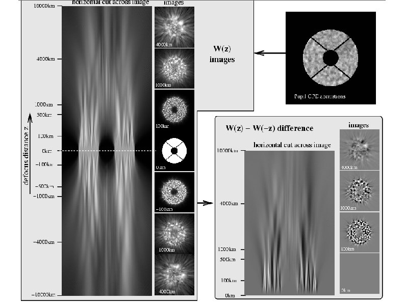
Curvature WFS Light propagation turns phase into amplitude (similar to scintillation) Lenslet array used to inject light into a series of fibers, which are connected to photoncounting Avalanche Photo. Diodes (APDs) 7

Curvature WFS Wavefront Signal. The optimal defocus distance at which the measured signal is strongest, is larger for lower spatial frequencies. For high spatial frequencies the linear domain extends to ~ 500 km. 8

Reconstruction Algorithm 1 0

Reconstruction Algorithm For faster reconstruction: (1) bin down data to low resolution and run iterative algorithm (2) expand solution to full resolution and run a small number of iterations (3) Speed up convergence by injecting derivative between iterations Iterative loop is slow, but: - Linear algorithm can give fast low sensitivity estimate used as starting point - Locally linear (within 1 rad) - Becomes linear if aberration < 1 rad (valid for high performance AO closed loop) Faster hardware coming online (GPUs) 1 1

Wavefront sensing at the diffraction limit of the telescope

Computer Simulations showing contrast gain with high sensitivity WFS (non-linear curvature) m ~ 13 WFS Loop frequ RMS SR @ 0. 85 um SR @ 1. 6 um nl. Curv 260 Hz 101 nm 57% 85% SH - D/9 180 Hz 315 nm ~4% 22% SH - D/18 180 Hz 195 nm ~13% 56% SH - D/36 160 Hz 183 nm ~16% 60%3 1

"High Sensitivity Wavefront Sensing with a non-linear Curvature Wavefront Sensor", Guyon, O. PASP, 122, pp. 49 -62 (2010) 1 4

Sensitivity Wavefront sensor sensitivity: definition Sensitivity = how well each photon is used For a single spatial frequency (OPD sine wave in the pupil plane, speckle in the focal plane): Error (rad) = Sensitivity / sqrt( # of photons) IDEAL WFS: Sensitivity Beta = 1 (1 ph = 1 rad of error) At all spatial frequencies Non-ideal WFS: Beta > 1 (Beta x Beta ph = 1 rad of error)

Wavefront sensors ''sensitivities'' in linear regime with full coherence (Guyon 2005) Square root of # of photons required to reach fixed sensing accuracy plotted here for phase aberrations only, 8 m telescope. Tuned for maximum sensitivity at 0. 5”from central star. Figure above shows sensitivity (y axis) as a function of pupil spatial frequency (x axis). Pupil spatial frequency = angular separation in focal plane. ALL wavefront sensor options have very good sensitivity at the spatial frequency defined by the WFS sampling SOME wavefront sensors loose sensitivity at low spatial frequencies (red), other do not (blue)

Sensitivity compared with other schemes 1 7

Performance gain for Ex. AO on 8 -m telescopes "High Sensitivity Wavefront Sensing with a non-linear Curvature Wavefront Sensor”, Guyon, O. PASP, 122, pp. 49 -62 (2010) Large gain at small angular separation: ideal for Ex. AO 1 8

Wavefront sensing at the sensitivity limit imposed by the telescope diffraction limit Seeing limited wavefront sensing (what we do now) Example: SH WFS Diffraction limited wavefront sensing (what needs to be done for Ex. AO) Examples: Pyramid (non-modulated), non-linear curvature Tip-tilt example (same argument applicable to other modes): With low coherence seeing-limited WFS, σ2 ~ 1/D 2 (more photons) Ideally, one should be able to achieve: σ2 ~ 1/D 4 (more photons + smaller λ/D) This makes a big difference for Extreme-AO on large telescopes For Tip-Tilt, SHWFS on ELT is 40000 x less sensitive than diffractionlimited WFS (11. 5 mag) Similar gain on other low order modes 1 9

Chromaticity 2 0

Chromaticity 2 1

Chromaticity compensation Simulation results Monochromatic algorithm Polychromatic data 2 2

Chromaticity compensation with chromatic optics 2 3

Optical implementation Better solution (suggested by Marcos Van Dam): split 4 beams according to wavelength with dichroics → mitigates (solves ? ) chromaticity issue (to be simulated and validated) 2 4

Faint source regime 2 5

Extended sources Extended source: → no diffraction limited speckles → sensitivity loss Example: seeing-limited source (Laser Guide Star) → no gain beyond SH WFS However, nl. CWFS should be beneficial for extended source with fine structure → simultaneous wavefront + source estimation required 2 6

Lab validation Dual arm: nl. CWFS + SHWFS nl. CWFS camera Light source SHWFS camera 2 7

Wavefront reconstruction 2 8

Sensitivity measurement using lab data 2 9

Conclusions The nl. CWFS concept offers high sensitivity without requiring high quality wavefront → attractive for adaptive optics Can fully exploit the telescope diffraction limit in a wide range of conditions – Star brighter that m. V~15 – Natural guide star (or possibly extended object with structure) → nl. CWFS greatly improves sensitivity for NGS, and for low-order aberrations, makes NGS as good a target as LGS ~1000 x to 10000 x brighter on large telescopes Challenges are computing power for reconstruction and chromaticity Lab demonstration ongoing, plans to install on ground-based telescope For more info on the concept: "High Sensitivity Wavefront Sensing with a non-linear Curvature Wavefront Sensor", Guyon, O. PASP, 122, 3 pp. 49 -62 (2010) 0